The original example is from exceldashboardtemplates.com, in a blog post by SteveEqualsTrue: http://www.exceldashboardtemplates.com/how-to-make-an-excel-project-status-spectrum-chart/
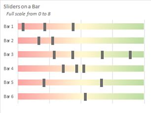
I came up with this, with up to four markers per category:
The howto with images is way too long for me to post here. The file may be downloaded from Dropbox:
https://www.dropbox.com/s/z6vh89zta81bl4f/sliders_on_a_bar.xlsx?dl=0
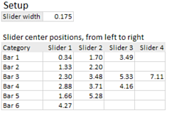
I setup the data like this. The top left cell, with the word "Setup", is C25:
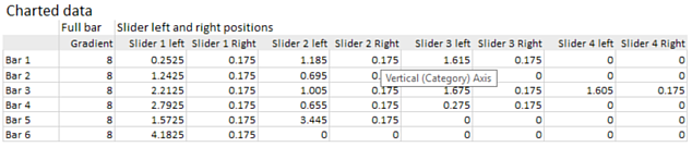
The charted data was setup like this, with the words "Charted data" in I25:
The Slider 1 left formula:
=(D30 <> "") * (D30 - 0.5 * SliderWidth)
This formula is equivalent to:
=IF(D30<>"", D30-0.5*SliderWidth, 0)
Slider 2 left formula:
=(E30 <> "") * (E30 - SUM(K28:L28) - 0.5 * SliderWidth)
Slider 3 and Slider 4 left formulas are similar to the Slider 2 left formula.
The Slider
N formulas merely copy the Slider width from cell D26.
This is the howto, without images:
- Determine full-scale maximum for the bars and enter that value in Charted Data: Gradient, J25:J30. I used a zero to eight scale, just as in the original.
- Enter a value for the slider width. You may change this value at any time. Good starting values seem to be in the 0.15 to 0.25 range. Higher values give thicker sliders.
- Enter the center positions for the sliders in D27:G32. If you don't want a particular slider, leave that cell blank. The Charted data cells will fill by formula. The formulas calculate where the left and right edges of each thumb should appear.
- Select I24:R30 and insert a stacked bar chart. With the chart selected, go to Chart Tools >> Design and click on Switch Row / Column.
- From the Plus-icon next to the chart, click on the right pointing arrow next to "Axes". Place a checkmark in all four checkboxes. All these axes will probably need to be reformatted.
- The primary horizontal axis is at the top. Change the maximum bounds of both axes to equal the value entered in Charted data: Gradient, cells J25:J30. Format both vertical axes to "Categories in reverse order".
- Delete the right axis and one of the horizontal axes. I chose to delete the top axis. The legend was annoying me—I removed it in this step. You may find it useful to keep the legend for now, postponing its removal till later.
- Format all "Slider Left" series to no fill, no line. These are the orange, yellow, green, and brown series in the images above. Format all the "Slider right series to the color or colors of your choice. I chose a dark gray.
- For the Gradient series, we want a gradient fill. In the formatting pane, set the fill to "Gradient", and the "Type" to "Radial". We use three gradient stops, with the center stop positioned at 50%.
- The stops are in reverse order from the display of our chart. The left stop controls the right-hand color, the right stop controls the left color.
- Adjust the gap widths. I set the gap for the Gradient series to 125%, the sliders gap to 70%.
- Add your finishing touches. I found that deleting the remaining, the bottom, horizontal axis messed up the whole chart's scale. Perhaps because it's a secondary axis? I ended up giving it a custom number format to hide it.
I hope I've been clear with the instructions, with images, included in the Excel file. I'll gladly answer any questions.
")


