Need help grouping while also eliminating duplicates

[MNik]

Hi All,

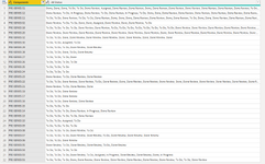
I had another questions solved in a previous post here. Need help with statement to return a value based a cell containing multiple values

However, I did not realize that the group by statement that I had originally used did not eliminate duplicate values, it only hid them, which is not allowing me to make a one to many relationship. Is it possible to achieve results like in the attached screenshot while removing all duplicates from the "Components" field?

Thanks in advance!

 

[KRice]

Does your original table consist of two columns (Components and Status), and each Status cell contains only one entry, either "To Do", "Assigned", "In Progress", "Repeat Validation", "Backlog", "Done Review", or "Done"? If so, I would consider going about this differently: using Power Query to Pivot the original data into a table whose column headings are To Do, Assigned,..and the body of the table consists of the count.

 

[KRice]

In the post you linked to above, you mentioned 'any combination of "To Do", "Assigned", "In Progress", "Repeat Validation", "Backlog", "Done Review", or "Done", I would like it to return a value of 2'. Does this mean any combination of two of more of the status categories? If so, then is it possible for some Components to have neither a 1, 2, or 3 (e.g., suppose a component appears only once with a status of "In progress")...or is that not possible? Regarding you comment about duplicates, I'm not sure I understand the issue. Suppose you have this source table (a set of 9 components appearing two times, with some variation on status categories):

MrExcel_20220913b.xlsx
	A	B
1	Components	All Status
2	PRE-SERIES 31	To Do
3	PRE-SERIES 12	Assigned
4	PRE-SERIES 11	In Progress
5	PRE-SERIES 02	Repeat Validation
6	PRE-SERIES 18	Backlog
7	PRE-SERIES 20	Done Review
8	PRE-SERIES 32	Done
9	PRE-SERIES 33	Assigned
10	PRE-SERIES 13	To Do
11	PRE-SERIES 31	To Do
12	PRE-SERIES 12	Assigned
13	PRE-SERIES 11	In Progress
14	PRE-SERIES 02	Repeat Validation
15	PRE-SERIES 18	Backlog
16	PRE-SERIES 20	Done Review
17	PRE-SERIES 32	Done
18	PRE-SERIES 33	To Do
19	PRE-SERIES 13	Done
Sheet1

This M Code in Power Query transforms the table, grouping like Components and then pivoting the table to count the number of items for each Status Category. Then the number of non-zero items are summed across each row (Values column) and logic is applied to assign 1, 2, or 3 (or 0 if none of the other conditions are met).

let
    Source = Excel.CurrentWorkbook(){[Name="Table1"]}[Content],
    #"Changed Type" = Table.TransformColumnTypes(Source,{{"Components", type text}, {"All Status", type text}}),
    #"Grouped Rows" = Table.Group(#"Changed Type", {"Components"}, {{"CGroups", each _, type table [Components=nullable text, All Status=nullable text]}}),
    #"Added Index" = Table.AddIndexColumn(#"Grouped Rows", "Index", 0, 1, Int64.Type),
    #"Expanded CGroups" = Table.ExpandTableColumn(#"Added Index", "CGroups", {"All Status"}, {"All Status"}),
    #"Pivoted Column" = Table.Pivot(#"Expanded CGroups", List.Distinct(#"Expanded CGroups"[#"All Status"]), "All Status", "Index", List.NonNullCount),
    #"Sorted Rows" = Table.Sort(#"Pivoted Column",{{"Components", Order.Ascending}}),
    #"Added Custom1" = Table.AddColumn(#"Sorted Rows", "Values", each List.Count( List.Select( { [To Do], [Assigned], [In Progress], [Repeat Validation], [Backlog], [Done Review], [Done] } /*Record.FieldValues(_)*/,
                each _ >0 ) ) ),
    #"Added Conditional Column" = Table.AddColumn(#"Added Custom1", "Results Code", each if [Values] > 1 then 2 else if [Values] = 1 and [To Do] > 0 then 1 else if [Values] = 1 and [Done] > 0 then 3 else 0)
in
    #"Added Conditional Column"

The output table, for now, looks like this...but it can be trimmed down in Power Query after you confirm this is what you want.

MrExcel_20220913b.xlsx
	A	B	C	D	E	F	G	H	I	J
1	Components	To Do	Assigned	In Progress	Repeat Validation	Backlog	Done Review	Done	Values	Results Code
2	PRE-SERIES 02	0	0	0	2	0	0	0	1	0
3	PRE-SERIES 11	0	0	2	0	0	0	0	1	0
4	PRE-SERIES 12	0	2	0	0	0	0	0	1	0
5	PRE-SERIES 13	1	0	0	0	0	0	1	2	2
6	PRE-SERIES 18	0	0	0	0	2	0	0	1	0
7	PRE-SERIES 20	0	0	0	0	0	2	0	1	0
8	PRE-SERIES 31	2	0	0	0	0	0	0	1	1
9	PRE-SERIES 32	0	0	0	0	0	0	2	1	3
10	PRE-SERIES 33	1	1	0	0	0	0	0	2	2
Table1

 

[MNik]

My apologies if my original post wasn't clear as to what I am trying to accomplish.

It is possible for a component to have only one status, but most have multiple. The way the data is captured each component can have multiple status's due to having a ticket created for each logged incident in our system. Think of it like an IT ticketing system where a single user can have one or multiple tickets they have created.

Right now, I have the data grouped by "Components" which resulted in the "All Status" column showing each different status relating to the component. I was not aware that when grouping, it did not eliminate duplicates, but more so just hid them. Due to to the duplicate not being eliminated, connecting data sets is resulting in a many to many relationship

My goal is to create a column with values of 1, 2, or 3, which can then be used to create a red, yellow, or green measure based on that number.

Here is how I am trying to assign a number:

If the component only contains "To Do", even if multiple, then 1
If a component has any of the other status or combination of status's including "To" or "Done" then assign a 2.
If the component only contains "Done", even if multiple, then 3

Does that make more sense?

 

[KRice]

Yes, I think I follow you. For the notional source table in my last post, would columns A & J below represent what you want to see as results:

MrExcel_20220913b.xlsx
	A	B	C	D	E	F	G	H	I	J
1	Components	To Do	Assigned	In Progress	Repeat Validation	Backlog	Done Review	Done	Values	Results Code
2	PRE-SERIES 02	0	0	0	2	0	0	0	1	2
3	PRE-SERIES 11	0	0	2	0	0	0	0	1	2
4	PRE-SERIES 12	0	2	0	0	0	0	0	1	2
5	PRE-SERIES 13	1	0	0	0	0	0	1	2	2
6	PRE-SERIES 18	0	0	0	0	2	0	0	1	2
7	PRE-SERIES 20	0	0	0	0	0	2	0	1	2
8	PRE-SERIES 31	2	0	0	0	0	0	0	1	1
9	PRE-SERIES 32	0	0	0	0	0	0	2	1	3
10	PRE-SERIES 33	1	1	0	0	0	0	0	2	2
Table1

This approach groups by Component name and counts and categorizes those counts by status. The output table could be reduced to just two columns (A and J) for subsequent use, and the results table would be delivered without duplicate Components. I modified the last line of M Code shown previously to adjust the rule for delivering "2":

let
    Source = Excel.CurrentWorkbook(){[Name="Table1"]}[Content],
    #"Changed Type" = Table.TransformColumnTypes(Source,{{"Components", type text}, {"All Status", type text}}),
    #"Grouped Rows" = Table.Group(#"Changed Type", {"Components"}, {{"CGroups", each _, type table [Components=nullable text, All Status=nullable text]}}),
    #"Added Index" = Table.AddIndexColumn(#"Grouped Rows", "Index", 0, 1, Int64.Type),
    #"Expanded CGroups" = Table.ExpandTableColumn(#"Added Index", "CGroups", {"All Status"}, {"All Status"}),
    #"Pivoted Column" = Table.Pivot(#"Expanded CGroups", List.Distinct(#"Expanded CGroups"[#"All Status"]), "All Status", "Index", List.NonNullCount),
    #"Sorted Rows" = Table.Sort(#"Pivoted Column",{{"Components", Order.Ascending}}),
    #"Added Custom1" = Table.AddColumn(#"Sorted Rows", "Values", each List.Count( List.Select( { [To Do], [Assigned], [In Progress], [Repeat Validation], [Backlog], [Done Review], [Done] } /*Record.FieldValues(_)*/,
                each _ >0 ) ) ),
    #"Added Conditional Column" = Table.AddColumn(#"Added Custom1", "Results Code", each if [Values] = 1 and [To Do] > 0 then 1 else if [Values] = 1 and [Done] > 0 then 3 else if [Values] >= 1 then 2 else 0)
in
    #"Added Conditional Column"

 

[MNik]

Yes, this looks like it captures what I am looking for. What will be the best way to move the power query you provided into power bi?

 

[KRice]

If you're doing this in Power BI, it might make more sense to build the query from within Power BI. Just connect to your workbook with the raw source table that resembles the first one shown in my post #3. I believe Home > Excel Workbook will make that connection. After you navigate to the file and identify the worksheet, you would choose "Transform Data", which will launch Power Query from Power BI. You should see the raw table from your worksheet. Then go to View > Advanced Editor and splice in my code:

let
    Source = Excel.CurrentWorkbook(){[Name="Table1"]}[Content],
    #"Changed Type" = Table.TransformColumnTypes(Source,{{"Components", type text}, {"All Status", type text}}),
    #"Grouped Rows" = Table.Group(#"Changed Type", {"Components"}, {{"CGroups", each _, type table [Components=nullable text, All Status=nullable text]}}),
    #"Added Index" = Table.AddIndexColumn(#"Grouped Rows", "Index", 0, 1, Int64.Type),
    #"Expanded CGroups" = Table.ExpandTableColumn(#"Added Index", "CGroups", {"All Status"}, {"All Status"}),
    #"Pivoted Column" = Table.Pivot(#"Expanded CGroups", List.Distinct(#"Expanded CGroups"[#"All Status"]), "All Status", "Index", List.NonNullCount),
    #"Sorted Rows" = Table.Sort(#"Pivoted Column",{{"Components", Order.Ascending}}),
    #"Added Custom1" = Table.AddColumn(#"Sorted Rows", "Values", each List.Count( List.Select( { [To Do], [Assigned], [In Progress], [Repeat Validation], [Backlog], [Done Review], [Done] } /*Record.FieldValues(_)*/,
                each _ >0 ) ) ),
    #"Added Conditional Column" = Table.AddColumn(#"Added Custom1", "Results Code", each if [Values] = 1 and [To Do] > 0 then 1 else if [Values] = 1 and [Done] > 0 then 3 else if [Values] >= 1 then 2 else 0),
    #"Removed Other Columns" = Table.SelectColumns(#"Added Conditional Column",{"Components", "Results Code"})
in
    #"Removed Other Columns"

You will probably use my code beginning with the 3rd line ( #"Grouped Rows") and down. You may want to edit the existing code in the query on the 2nd line (#"Changed Type") to rename the columns to something other than the defaults "Column1" and "Column2". Also note that when you splice in the code, each row needs to end with a comma (,), except for the last one before "in". So when the splicing is done, you may need to add a comma to the last existing row then paste new code. Also confirm that the embedded reference to the previous step matches the name of the previous step (the text appearing to the left of the equals sign). This is a common issue where the last step of existing code and the first step of newly pasted code have mismatched names. In the version of the code shown here, I've added a last step to select only two columns (Component and Results Code).

 

[MNik]

Perfect! Thank you so much for your help!

 

[KRice]

You're welcome...I'm happy to help.