Need help transposing/reorganizing data

[MajesticAmy84]

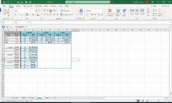
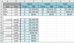
Hello, I have this spreadsheet that is arranged like cells A1:H5, and I'm trying to put that information in a spreadsheet that is arranged like cells A7:D15. I tried transposing it, but it doesn't come out the way I want it to. I've also tried just doing this all the way down in the C column and dragging it down:
=C3
=E3
=G3
=C4
=E4
=G4
...but Excel can't seem to figure out the pattern. I've also played around with the OFFSET function, but I can't get that to work either. It still doesn't follow my pattern.

There must an easier way to do this than just moving all of it manually. I have a year's worth of data. I've never used macros or VBA before so I'd rather avoid that unless it's the only possible way.

Does anyone have a solution?

 

[sandy666]

use XL2BB to post your source data (without merged cells) and expected result (not a pictures)

 

[Peter_SSs]

Welcome to the MrExcel board!

See if this would help.

21 01 30.xlsm
	B	C	D	E	F	G	H	I	J	K	L	M
1		Check		Credit		Cash
2	Date	Trans	$$$	Trans	$$$	Trans	$$$				Trans	$$$
3	1/02/2018	9	$8.00	5	$5.00	8	$6.00		1/02/2018	Check	9	$8.00
4	1/03/2018	1	$4.00	9	$7.00	6	$3.00			Credit	5	$5.00
5	1/04/2018	9	$5.00	8	$6.00	6	$2.00			Cash	8	$6.00
6									1/03/2018	Check	1	$4.00
7										Credit	9	$7.00
8										Cash	6	$3.00
9									1/04/2018	Check	9	$5.00
10										Credit	8	$6.00
11										Cash	6	$2.00
12
13
14
Rearrange

Cell Formulas
Range	Formula
J3:J14	J3	=IF(K3="Check",INDEX(B$3:B$1000,COUNTIF(K$3:K3,"Check")),"")
K3:K14	K3	=IF(ROWS(K$3:K3)>COUNT(B$3:B$1000)*3,"",INDEX({"Cash","Check","Credit"},MOD(ROWS(K$3:K3),3)+1))
L3:L14	L3	=IF(K3="","",INDEX(C$3:H$1000,COUNTIF(K$3:K3,K3),MATCH(K3,C$1:H$1,0)))
M3:M14	M3	=IF(K3="","",INDEX(C$3:H$1000,COUNTIF(K$3:K3,K3),MATCH(K3,C$1:H$1,0)+1))

 

[MajesticAmy84]

Welcome to the MrExcel board!

See if this would help.

21 01 30.xlsm
	B	C	D	E	F	G	H	I	J	K	L	M
1		Check		Credit		Cash
2	Date	Trans	$$$	Trans	$$$	Trans	$$$				Trans	$$$
3	1/02/2018	9	$8.00	5	$5.00	8	$6.00		1/02/2018	Check	9	$8.00
4	1/03/2018	1	$4.00	9	$7.00	6	$3.00			Credit	5	$5.00
5	1/04/2018	9	$5.00	8	$6.00	6	$2.00			Cash	8	$6.00
6									1/03/2018	Check	1	$4.00
7										Credit	9	$7.00
8										Cash	6	$3.00
9									1/04/2018	Check	9	$5.00
10										Credit	8	$6.00
11										Cash	6	$2.00
12
13
14
Rearrange

Cell Formulas
Range	Formula
J3:J14	J3	=IF(K3="Check",INDEX(B$3:B$1000,COUNTIF(K$3:K3,"Check")),"")
K3:K14	K3	=IF(ROWS(K$3:K3)>COUNT(B$3:B$1000)*3,"",INDEX({"Cash","Check","Credit"},MOD(ROWS(K$3:K3),3)+1))
L3:L14	L3	=IF(K3="","",INDEX(C$3:H$1000,COUNTIF(K$3:K3,K3),MATCH(K3,C$1:H$1,0)))
M3:M14	M3	=IF(K3="","",INDEX(C$3:H$1000,COUNTIF(K$3:K3,K3),MATCH(K3,C$1:H$1,0)+1))

Yes that seems to work! Thank you!

 

[Peter_SSs]

You're welcome. Thanks for the follow-up.