Need help with dynamic range selection in formula

[randyharris]

This one is stumping me, would appreciate some ideas.

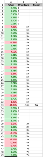
I have three columns:

• Column A contains monthly return % figures
• Column B tracks the drawdown%
• Column C indicates when the drawdown hits 15% or more (negative)

I'm hoping for a single formula in column B which adjusts the starting point based on the "Yes" indicators in column C.

The drawdown formula starting in cell B2 goes from the range $A$1:A1, and as the formula goes down it goes from $A$1:current row.

What I'm trying to do is whenever column C shows "Yes", then then in column B, the row after the "Yes" would instead of starting from $A$1, would start from the row after the "Yes" Row.

In the attached picture, cell B34, I would want it to be looking at the range $A$34:A34, instead of $A$1:A34. And if cell C50 had a "Yes", then B50 would be looking at the range $A$51:A51

Was thinking about maybe incorporating a check for the YES and if there, using the Offset formula, but couldn't figure it out.

 

[steve the fish]

Your example doesnt make complete sense to me. You use row 1 with the formula in row 2 then later on you use the same row for where you want to look and the formula. However you can use some sort of index setup. Ive used it with a SUM formula here as an example:

=SUM(INDEX($A$1:A1,IF(ISNUMBER(MATCH("yes",$C$1:C1,0)),LOOKUP("yes",$C$1:C1,ROW($C$1:C1)),1)):INDEX($A$1:A1,ROW(A1)))

This will move the sum range based on seeing yes in column C. Use the evaluate formula tool to see what its doing as it moves down the column.

 

[randyharris]

Steve the Fish (haha)

Sorry I didn't explain it as clearly as it should have been. Your formula is really close, but I'm having trouble adapting it.

If you look at the image below, the formula in Column B is a VBA function, drawdown.

• B2 is looking at the range of $A$2:A2
• B3 looks at the drawdown range of $A$2:A3, and so on down the column

The Trigger column C is what I hope to use the name the drawdown range dynamic.

• Row 33 is a Trigger "Yes", this means that
• cell B34, seeing the Trigger in C33, it would change the range it looks at from $A$2:A34 to $A$34:B34

So the drawdown formula in Column B, I'm hoping to start at the current row instead of A2 when there is a Yes in column C, (one row above the current formula in column B's row")

 

[steve the fish]

Try this:

=DRAWDOWN(INDEX($A$2:A2,IFERROR(LOOKUP(2,1/($C$2:C2="yes"),ROW($C$2:C2)-1),1)):INDEX($A$2:A2,ROW(A2)-1))