Need help with formula.. possibly an array?

[x8xviperx6x]

First off sorry for not being able to insert as an excel table I couldn't figure out how to input such a large table..

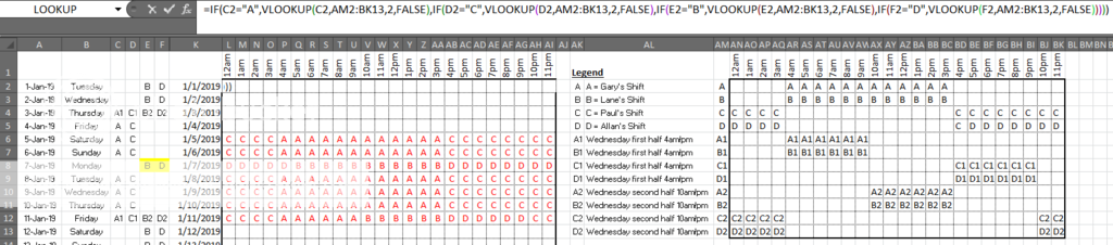
I’m having issues coming up with a formula that will get theresults I need. Below is an image of the data on my sheet.


What is displayed in column A is the days of the year.Column C is the shift codes that each shift works. If blank they are off. Inthe array AM2:BK13 displays what each shift hours are in accordance to theshift code.


Columns C:F can change daily, its controlled by datavalidation using a drop down menu changed by user input.


The problems is L:AI columns for the entire year needs to autopopulate as the user changes the schedule. Thus resulting in an easy copy pasteschedule.


In cell L2 I’ve tried several IF formulas with a vlookupand/or Index/matching and the problem is vlookup and index matching result in a0 when there is a blank in the array am2:bk13 thus ending the formulaprematurely.


L2 example formula:


=IF(C2="A",VLOOKUP(C2,AM2:BK13,2,FALSE),IF(D2="C",VLOOKUP(D2,AM2:BK13,2,FALSE),IF(E2="B",VLOOKUP(E2,AM2:BK13,2,FALSE),IF(F2="D",VLOOKUP(F2,AM2:BK13,2,FALSE)))))


But my formula results in a 0 when it gets to the if(e2=”B”…results in true returns a 0, and doesn’t continue to the last lookup. Which I don’tunderstand why it’s a zero instead of blank for that hr range, and continue onto the last IF statement.


I thought about adding the AND statement for the AND(e2=”B”,am2<>””)but that is a lot more input to the formula. Example: The letters in RED arethe result I need for the auto population.




I'm going to guess I need to start researching array formulas...
Any help would be greatly appreciated, thanks in advanced!

 

[DanteAmor]

In theory, if the result of looking for E2 is white, then you would have to put another IF, so that you can continue with the F2 search, for example:

=IF(C2="A",VLOOKUP(C2,AM2:BK13,2,FALSE),IF(D2="C",VLOOKUP(D2,AM2:BK13,2,FALSE),
IF(E2="B",
IF(VLOOKUP(E2,AM2:BK13,2,FALSE)<>"",
VLOOKUP(E2,AM2:BK13,2,FALSE),
IF(F2="D",
VLOOKUP(F2,AM2:BK13,2,FALSE)))))

You should also do it for C2 and D2

Try the following:

Book1
	A	B	C	D	E	F	L	M	N	AL	AM	AN
1
2					B	D	D				A
3											B
4											C	C
5											D	D
6											A1
7											B1
8											C1
Hoja3

Cell Formulas
Range	Formula
L2	=INDEX(AN1:AN7,SUMPRODUCT(((AM2:AM13=C2)+(AM2:AM13=D2)+(AM2:AM13=E2)+(AM2:AM13=F2))*(AN2:AN13<>"")*(ROW(AN2:AN13))))

 

[Aladin Akyurek]

Just considering the formula with VLOOKUP you posted...

=IF(C2="A",VLOOKUP(C2,AM2:BK13,2,FALSE),IF(D2="C",VLOOKUP(D2,AM2:BK13,2,FALSE),IF(E2="B",VLOOKUP(E2,AM2:BK13,2,FALSE),IF(F2="D",VLOOKUP(F2,AM2:BK13,2,FALSE)))))

can be rewritten as

=VLOOKUP(LOOKUP(REPT("z",255),C2:F2),

AM2:BK13,2,0)

assuming that C2:F2 contains just one value at any time.​

_{^{<strike>
</strike>}}​

 

[x8xviperx6x]

In theory, if the result of looking for E2 is white, then you would have to put another IF, so that you can continue with the F2 search, for example:

=IF(C2="A",VLOOKUP(C2,AM2:BK13,2,FALSE),IF(D2="C",VLOOKUP(D2,AM2:BK13,2,FALSE),
IF(E2="B",
IF(VLOOKUP(E2,AM2:BK13,2,FALSE)<>"",
VLOOKUP(E2,AM2:BK13,2,FALSE),
IF(F2="D",
VLOOKUP(F2,AM2:BK13,2,FALSE)))))

You should also do it for C2 and D2

Try the following:

	A	B	C	D	E	F	L	M	N	AL	AM	AN
1
2					B	D	D				A
3											B
4											C	C
5											D	D
6											A1
7											B1
8											C1

<colgroup><col><col><col><col><col><col><col><col><col><col><col><col><col></colgroup><thead>
</thead><tbody>
</tbody>

Hoja3​

Worksheet Formulas Cell Formula L2 =INDEX(AN1:AN7,SUMPRODUCT(((AM2:AM13=C2)+(AM2:AM13=D2)+(AM2:AM13=E2)+(AM2:AM13=F2))*(AN2:AN13<>"")*(ROW(AN2:AN13)))) <thead> </thead><tbody> </tbody>

<tbody>
</tbody>

Yes, that is correct, for it to continue the search i'd need to add IF statements to have it continue each column.
I tested out your index formula and it works up until the 4th row it gives me #REF errors, that's when all four shifts work a 6hr portion of the day and it is identified as shift A1 is first half, etc. Although A1 works B thru D show #REF .

 

[x8xviperx6x]

Just considering the formula with VLOOKUP you posted...

=IF(C2="A",VLOOKUP(C2,AM2:BK13,2,FALSE),IF(D2="C",VLOOKUP(D2,AM2:BK13,2,FALSE),IF(E2="B",VLOOKUP(E2,AM2:BK13,2,FALSE),IF(F2="D",VLOOKUP(F2,AM2:BK13,2,FALSE)))))

can be rewritten as

=VLOOKUP(LOOKUP(REPT("z",255),C2:F2),

AM2:BK13,2,0)

assuming that C2:F2 contains just one value at any time.​

_{^{<strike>
</strike>}}​

I will have to test that out, that is significantly shorter, unfortunately at all times column C2:F2 will have 2 or more letters

 

[DanteAmor]

Sorry, In the first formula I omitted change 7 by 13

You have to check the relative and absolute part of the cells.


=INDEX($AN$1:$AN$13,SUMPRODUCT((($AM$2:$AM$13=C2)+($AM$2:$AM$13=D2)+($AM$2:$AM$13=E2)+($AM$2:$AM$13=F2))*($AN$2:$AN$13<>"")*(ROW($AN$2:$AN$13))))

Try again

 

[x8xviperx6x]

Sorry, In the first formula I omitted change 7 by 13

You have to check the relative and absolute part of the cells.


=INDEX($AN$1:$AN$13,SUMPRODUCT((($AM$2:$AM$13=C2)+($AM$2:$AM$13=D2)+($AM$2:$AM$13=E2)+($AM$2:$AM$13=F2))*($AN$2:$AN$13<>"")*(ROW($AN$2:$AN$13))))

Try again

Flawless, I overlooked that too! Brilliant formula, thank you very much!

 

[Aladin Akyurek]

Did you try post #3 at all?

 

[DanteAmor]

Flawless, I overlooked that too! Brilliant formula, thank you very much!

I'm glad to help you. I appreciate your kind comments.

 

[Aladin Akyurek]

I will have to test that out, that is significantly shorter, unfortunately at all times column C2:F2 will have 2 or more letters

Are they prioritized? If not, are you intending to sum the results? If the latter, the results must be numeric...