Need help with using IF(ISNA(VLOOKUP....) to return value of cell or "needs setup"

[kznmrexcel]

Hi, everybody,
I know how to use IF(ISNA(VLOOKUP....) to return message A or message B, but I'd like to return the actual content from the cell looked up if it's there.

Right now, I have this formula:
=IF(ISNA(VLOOKUP(B2,aeriesLoginDate!$A:$G,5,FALSE)), "Needs setup", "CBDC")

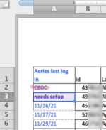
Instead of "CBDC" I would like the exact date that appears from the other sheet if a date is present. The rest of this formula does the job. I'm including a screenshot. A2 shows the problem of using the formula shown above. A3, A4, A5, and A6, show what I want returned if possible. (A3 also has conditional formatting for the "needs setup," a separate topic. I already know how to do that.)

I appreciate any help with this.

Thanks,
K.

 

[jasonb75]

Sounds like you just want

=IFERROR(VLOOKUP(B2,aeriesLoginDate!$A:$G,5,FALSE),"Nedds setup")

ISNA(VLOOKUP is a pointless waste of system resource processing the precedent range, you should use ISNA(MATCH( on the left hand column if you only want to test for presence.

 

[kznmrexcel]

@jasonb75 , that is very helpful. I have a follow-up question:
Is there some way to deal with a zero when it's listed instead of a date? A few students are listed with a zero [0] instead of blank, N/A or not being listed. When I use the formula you gave me, it returns 1/0/00 if the value on the aeriesLoginDate worksheet is 0. I would like any student with "0" under last login OR any student with N/A or not listed to return as "needs setup." ??

 

[jasonb75]

This will return anything that doesn't contain a valid date as "Needs setup", does that work?

=IFERROR(1/(1/VLOOKUP(B2,aeriesLoginDate!$A:$G,5,FALSE)),"Needs setup")

 

[kznmrexcel]

That looks perfect! Thank you.
BTW, if you have time (and only if), please share what the function is of the (1/(1/VLOOKUP...) I've never seen this before.
Thanks so much!

 

[kznmrexcel]

I appreciate your help!

 

[jasonb75]

The 1/(1/vlookup part forces the formula to return an error when the result is not a number other than 0.

Dividing 1 by any non 0 number will still give a value, dividing 1 by the result of the first calculation returns to the original value. If the starting value was 0, text, or an error then it will trigger another error and the lookup result is ignored in favour of the error trap.

 

[kznmrexcel]

Good to know! Thank you so much!