Hello,
I am in the process of making a scheduling system for an orthopedic floor. View 2 is a sheet that is printed out for medical staff so they can see which times patients (by room number) have appointments with therapy. I used an index match to search and return times based on room numbers. This has worked great but per the feedback I received I also need initials to be shown.
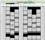
In view 1 you can see room numbers are always listed in the first cell of a 3 cell block. Initials are always listed below the room number. To find appointment times based on room number for PT's I have used the formula below. In the formula, PT is defined dynamically in the name manager via a macro to accommodate the constant change of staff schedules (Person 1, Person 2, etc). A similar method was used for OT.
=INDEX('Current Schedule'!$A$4:$A$47,SMALL(IF(ISNUMBER(MATCH(PT,A5,0)),MATCH(ROW(PT),ROW(PT)),""),ROWS('Current Schedule'!$Z$1:$Z$1))) - This returns the appointment time for room 6103 for PT in View 2.
I know there are several ways to do this but I need help modifying or using a different formula that will find the specified room number across a dynamic set of columns and return the cell below it (initials). Can anyone offer me feedback on how I can accomplish this task? The problem I am running in to is the initials are below room numbers instead of next to them. Thank you!
I am in the process of making a scheduling system for an orthopedic floor. View 2 is a sheet that is printed out for medical staff so they can see which times patients (by room number) have appointments with therapy. I used an index match to search and return times based on room numbers. This has worked great but per the feedback I received I also need initials to be shown.
In view 1 you can see room numbers are always listed in the first cell of a 3 cell block. Initials are always listed below the room number. To find appointment times based on room number for PT's I have used the formula below. In the formula, PT is defined dynamically in the name manager via a macro to accommodate the constant change of staff schedules (Person 1, Person 2, etc). A similar method was used for OT.
=INDEX('Current Schedule'!$A$4:$A$47,SMALL(IF(ISNUMBER(MATCH(PT,A5,0)),MATCH(ROW(PT),ROW(PT)),""),ROWS('Current Schedule'!$Z$1:$Z$1))) - This returns the appointment time for room 6103 for PT in View 2.
I know there are several ways to do this but I need help modifying or using a different formula that will find the specified room number across a dynamic set of columns and return the cell below it (initials). Can anyone offer me feedback on how I can accomplish this task? The problem I am running in to is the initials are below room numbers instead of next to them. Thank you!
")


