Need some help picking the right formula

[Ldbyers]

Hey everyone first time poster here.

I am struggling with finding the correct formula to use. I am looking to pull data from my Unavailable tab and place the data from Column D in either the Meeting, Break, Lunch, or Tech Issue (Columns C:F) as labeled on my All Rep Stats tab.

I need it to match up Names and Dates with each sheet to provide the time that was used in each "Aux" for that specific day.

I cant seem to get the reference correct to pull it by name and date. I'm only able to get it to pull by name. Can anyone help with this?

Thanks!


Unavailable tab

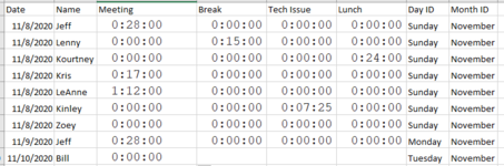
All Rep Stats Tab

 

[kweaver]

Welcome to Mr Excel. It would help us if you used XL2BB to post your data so that we don't have to retype it to test solutions.

Are the dates and names in the rep tab and you want to match those with the unavail data and insert the times in the appropriate cell?

 

[Ldbyers]

@kweaver ,thanks I wasn't aware of the XL2BB! I have it now and entered below the data from the two sheets. You were correct, I was wanting to match the Dates and Names to get the Time data inserted to the appropriate cell on the All Rep Stats tab.

Test Stats.xlsx
	A	B	C	D	E	F	G	H
1	Date	Name	Meeting	Break	Tech Issue	Lunch	Day ID	Month ID
2	11/8/2020	Jeff	0:28:00	0:00:00	0:00:00	0:00:00	Sunday	November
3	11/8/2020	Lenny	0:00:00	0:15:00	0:00:00	0:00:00	Sunday	November
4	11/8/2020	Kourtney	0:00:00	0:00:00	0:00:00	0:24:00	Sunday	November
5	11/8/2020	Kris	0:17:00	0:00:00	0:00:00	0:00:00	Sunday	November
6	11/8/2020	LeAnne	1:12:00	0:00:00	0:00:00	0:00:00	Sunday	November
7	11/8/2020	Kinley	0:00:00	0:00:00	0:07:25	0:00:00	Sunday	November
8	11/8/2020	Zoey	0:00:00	0:00:00	0:00:00	0:00:00	Sunday	November
9	11/9/2020	Jeff	0:28:00	0:00:00	0:00:00	0:00:00	Monday	November
10	11/10/2020	Bill	0:00:00				Tuesday	November
All Rep Stats

Cell Formulas
Range	Formula
D2:D8	D2	=SUMIFS(Unavailable!$D:$D,Unavailable!$C:$C,"Break",Unavailable!$B:$B,'All Rep Stats'!$B:$B)
E2:E8	E2	=SUMIFS(Unavailable!$D:$D,Unavailable!$C:$C,"Tech Issue",Unavailable!$B:$B,'All Rep Stats'!$B:$B)
F2:F8	F2	=SUMIFS(Unavailable!$D:$D,Unavailable!$C:$C,"Lunch",Unavailable!$B:$B,'All Rep Stats'!$B:$B)
D9	D9	=SUMIFS(Unavailable!$D:$D,Unavailable!$C:$C,"Break",$A:$A,$A:$A)
E9	E9	=SUMIFS(Unavailable!$D:$D,Unavailable!$C:$C,"Tech Issue",$A:$A,$A:$A)
F9	F9	=SUMIFS(Unavailable!$D:$D,Unavailable!$C:$C,"Lunch",$A:$A,$A:$A)
G2:G10	G2	=TEXT(A2,"DDDD")
H2:H10	H2	=TEXT(A2,"MMMM")
C2:C10	C2	=SUMIFS(Unavailable!$D:$D,Unavailable!$C:$C,"Meeting",Unavailable!$B:$B,'All Rep Stats'!$B:$B)

Test Stats.xlsx
	A	B	C	D
1	Date	Name	Aux Code	Time
2	11/8/2020	Jeff	Meeting	0:28:00
3	11/8/2020	Lenny	Break	0:15:00
4	11/8/2020	Kourtney	Lunch	0:24:00
5	11/8/2020	Kris	Meeting	0:17:00
6	11/8/2020	LeAnne	Meeting	1:12:00
7	11/8/2020	Kinley	Tech Issue	0:07:25
8	11/8/2020	Zoey	Tech Issue	0:00:00
9	11/9/2020	Jeff	Meeting	2:00:00
10	11/10/2020	Bill	Lunch	0:30:00
Unavailable

 

[Fluff]

How about in C2 copied down & across

=SUMIFS(Unavailable!$D:$D,Unavailable!$C:$C,C$1,Unavailable!$B:$B,$B2,Unavailable!$A:$A,$A2)

 

[Ldbyers]

@Fluff Awesome! Exactly what I needed!

 

[Fluff]

You're welcome & thanks for the feedback.