Need to add to existing formula Vlookup

[zone709]

Need to add on this formula. if Column E on detailed_view also matches has the name Monday. If Monday is there then return ,8

=IFERROR(VLOOKUP(@$D$8:$D$694, Detailed_View!$D$2:$P$395,8,0),"")

 

[Joe4]

I see a few issues with the first argument of your VLOOKUP function.
@$D$8:$D$694

1. The value you look up should be a single value, not a whole range of values.
2. Why do you have an "@" in front of the range? I don't think that should be there.
You are doing this in Excel, and not Google Sheets or an Open Source Document, right?

 

[zone709]

That range looks for the number in that row range to match the numbers on Detailed_View range. to return what's in ,8. This works i just need to add to it to use it in a different way.
If the word Monday is also in column E on Detailed row with the D columns matching then return the value in ,8

 

[zone709]

If i don't use @ it returns Spill. Not using a single number because it needs to look through the whole column D. I am using Excel 2016.

 

[Joe4]

I am a bit confused by what you are saying.
Are you really, really comfortable that you fully understand how VLOOKUP works?
If not, here is an explanation: MS Excel: How to use the VLOOKUP Function (WS)

Note that the first argument is typically a single value/cell reference, not a whole range.
If you have other values to look up, that cell reference will change as you copy the formula down the page.

If you try this formula, does it work for you?

=IFERROR(VLOOKUP(D8, Detailed_View!$D$2:$P$395,8,0),"")

If not please post a sample of your data, and your expected result, based off of that sample.

 

[Fluff]

I am using Excel 2016.

Not if you get #SPILL errors. You are using 365

 

[zone709]

ok I change it to 365 my profile. This formula works also, but i need it to only return if column E also on Detailed_view says Monday.

=IFERROR(VLOOKUP(D8, Detailed_View!$D$2:$P$395,8,0),"") This works like my other one but trying to add to it if Monday is in column E.

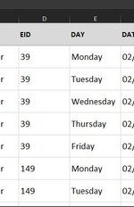
I have picture below. Trying to lookup the same number lets say its 39 and also E has to say Monday. Then is can return what's in ,8. Making sure the number matches and its Monday in E to return value in ,8

 

[Fluff]

Will you only ever have one row that meets both criteria?

 

[Joe4]

So, maybe something like this:

=IF(IFERROR(VLOOKUP(D8, Detailed_View!$D$2:$P$395,2,0),"")="Monday",IFERROR(VLOOKUP(D8, Detailed_View!$D$2:$P$395,8,0),""),"")

This is, of course, assuming that the value in column E is actually text, and not a date formatted to show Monday.

 

[zone709]

Yes Both D & D need to match then look for Monday in column E to return the right number in ,8