Need to average 3 non continuous cells based on text in a different cell

[rlange]

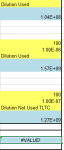
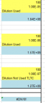
Hi. Thanks in advance! I'm trying to average cells F13, F20 and F27 but I only want to count any of them if their associated cell above it (F12, F19 and F26) contain the words "Dilution Used". If Dilution Used does not appear in F12, F19 or F26, then I don't want to include the associated cell in the average. Hopefully that makes sense. I've tried numerous functions and nothing produces a workable value. I usually get some sort of error. Help? Thank you!!!

Oh the average will go in cell F30

 

[jasonb75]

As long as no other cells in between could contain the text "Dilution used" then just do it as one range, the formula will ignore the other cells.

=AVERAGEIFS(F13:F27,F12:F26, "Dilution Used")

 

[rlange]

As long as no other cells in between could contain the text "Dilution used" then just do it as one range, the formula will ignore the other cells.

=AVERAGEIFS(F13:F27,F12:F26, "Dilution Used")

Hi Jason. Thank you! I put that formula in F30 and produced a new error: #DIV/0! Any ideas why that happened?

 

[jasonb75]

That would mean either no cells in F12:F26 contain the text "Dilution Used" or that the cells immediately above "Dilution Used" do not contain valid numbers.

 

[Peter_SSs]

or that the cells immediately above "Dilution Used" do not contain valid numbers.

below?

 

[jasonb75]

below?

I was looking at it downside up

 

[rlange]

That would mean either no cells in F12:F26 contain the text "Dilution Used" or that the cells immediately above "Dilution Used" do not contain valid numbers.

Hi Jason. Would numbers like these be invalid? There are numbers in the cells above and below the words "Dilution Used".

 

[rlange]

below?

Hi Peter. Yes, it's the cells immediately below the cells containing "Dilution Used" that need to be averaged. The numbers above aren't involved in the equation. Thanks!

 

[jasonb75]

As long as they are proper numbers in scientific format then it works, they look fine from the screen capture.

Check the cells with the text for typos, stray spaces, etc.

Book2
	F
10	100
11	1.00E-05
12	Dilution Used
13	1.04E+08
14
15
16
17	100
18	1.00E+06
19	Dilution Used
20	1.57E+09
21
22
23
24	100
25	1.00E+07
26	Dilution Not Used
27	1.27E+09
28
29
30	8.37E+08
Sheet4

Cell Formulas
Range	Formula
F30	F30	=AVERAGEIFS(F13:F27,F12:F26, "Dilution Used")

 

[Peter_SSs]

Quite likely an issue with your data. If still unresolved, post that sample data with XL2BB so we can copy exacly what you have rather than relying on us copying it manually from a picture.