Nested IF Formula help

[bburke73]

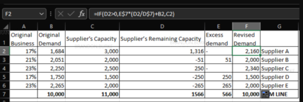
I want col F to calculate the reallocation of excess demand quantities shown in Col E to the suppliers who can take additional demand. But that reallocation must not exceed the max supplier capacity shown in Col C. And the SUM quantities in Col B must match the revised demand quantities SUM in Col F.

Best I can tell, I need a second IF statement to account for the multiple conditions I’m facing, but am struggling to put the formula construction together.

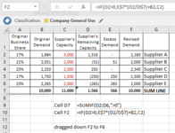
		Col A	Col B	Col C	Col D	Col E	Col F
Row 1		Original Business Share	Original Demand (QTY) Allocation	Supplier's Capacity	Supplier’s Remaining Capacity	Excess demand	Revised Demand (QTY) Allocation	Revised Demand allocation current formula in use
Row 2	Supplier A	17%	1,684	3,000	1,316	-	1,967	=IF(B5<C5,B5+(E$6/2),B5)
Row 3	Supplier B	21%	2,051	2,000	(51)	51	2,000
Row 4	Supplier C	23%	2,250	2,500	250	-	2,533
Row 4	Supplier D	17%	1,750	1,500	(250)	250	1,500
Row 5	Supplier E	23%	2,265	2,000	(265)	265	2,000
Row 6	SUM LINE		10,000	11,000	-	566	10,000

 

[Sufiyan97]

Hi
Welcome to MrExcel.

Can you some expected results, I am not getting what you want to achieve

 

[njimack]

On what basis are you calculating the revised qty for those suppliers with excess capacity?

 

[jtakw]

Hi,

Your sample result in F4 can not be correct, you have 2533 as revised allocation, but the Max capacity for that supplier is 2500 in C4.

See if this works for you:

Book3.xlsx
	A	B	C	D	E	F
1	Original Business Share	Original Demand (QTY) Allocation	Supplier's Capacity	Supplier’s Remaining Capacity	Excess demand	Revised Demand (QTY) Allocation
2	17%	1,684	3,000	1,316	-	2,160
3	21%	2,051	2,000	-51	51	2,000
4	23%	2,250	2,500	250	-	2,340
5	17%	1,750	1,500	-250	250	1,500
6	23%	2,265	2,000	-265	265	2,000
7		10,000	11,000	-	566	10,000
Sheet1041

Cell Formulas
Range	Formula
F2:F6	F2	=ROUND(MIN(C2,D2/SUMIF(D$2:D$6,">0",D$2:D$6)*E$7+B2),0)

 

[bburke73]

Hi,

Your sample result in F4 can not be correct, you have 2533 as revised allocation, but the Max capacity for that supplier is 2500 in C4.

See if this works for you:

Book3.xlsx
	A	B	C	D	E	F
1	Original Business Share	Original Demand (QTY) Allocation	Supplier's Capacity	Supplier’s Remaining Capacity	Excess demand	Revised Demand (QTY) Allocation
2	17%	1,684	3,000	1,316	-	2,160
3	21%	2,051	2,000	-51	51	2,000
4	23%	2,250	2,500	250	-	2,340
5	17%	1,750	1,500	-250	250	1,500
6	23%	2,265	2,000	-265	265	2,000
7		10,000	11,000	-	566	10,000
Sheet1041

Cell Formulas
Range	Formula
F2:F6	F2	=ROUND(MIN(C2,D2/SUMIF(D$2:D$6,">0",D$2:D$6)*E$7+B2),0)

Thanks jtakw! This solution is works great. Much obliged. I did end up using a different solution, much simpler actually, posted here for reference.

 

[jtakw]

Thanks jtakw! This solution is works great. Much obliged. I did end up using a different solution, much simpler actually, posted here for reference.

That's great, but that table in your latest post is Different than what you posted in OP (e.g. D7 in your OP is just "-", whereas, in your latest pic in Post #5, is 1566, where did That come from?), So I'm not so sure it's "much simpler", since you must have updated the table with more formulas.

 

[bburke73]

@jtakw: Apologies for the confusion. The 1,566 in D7 is the sum of the remaining supplier capacity; [=SUMIF(D2:D6,">0"]. Then I'm using the result in D7 for the calculation entered in cells F2:F6 [=IF(D2>0,D$7*(D2/D$7)+B5,C5)]; this formula construct solved my issue without the need for additional helper columns or the use of nested IFS.

 

[jtakw]

@jtakw: Apologies for the confusion. The 1,566 in D7 is the sum of the remaining supplier capacity; [=SUMIF(D2:D6,">0"]. Then I'm using the result in D7 for the calculation entered in cells F2:F6 [=IF(D2>0,D$7*(D2/D$7)+B5,C5)]; this formula construct solved my issue without the need for additional helper columns or the use of nested IFS.

The solution/formula in my Post #4 did not use Any helper cells, helper columns, or nested IFs, just to clarify.

So, basically, you've used D7 as a Helper Cell for your formula in F2:F6, which, if combined, your 2 formulas ( D7 and F2:F6 ) is basically the same Single formula as what I posted, but you've used an IF statement where I didn't.

Here would be my formula from Post #4 for F2:F6 with the D7 formula in place:

Book3.xlsx
	A	B	C	D	E	F
1	Original Business Share	Original Demand (QTY) Allocation	Supplier's Capacity	Supplier’s Remaining Capacity	Excess demand	Revised Demand (QTY) Allocation
2	17%	1,684	3,000	1,316	-	2,160
3	21%	2,051	2,000	-51	51	2,000
4	23%	2,250	2,500	250	-	2,340
5	17%	1,750	1,500	-250	250	1,500
6	23%	2,265	2,000	-265	265	2,000
7		10,000	11,000	1,566	566	10,000
Sheet1041

Cell Formulas
Range	Formula
F2:F6	F2	=MIN(C2,D2/D$7*E$7+B2)
D7	D7	=SUMIF(D2:D6,">0")

 

[bburke73]

The solution/formula in my Post #4 did not use Any helper cells, helper columns, or nested IFs, just to clarify.

So, basically, you've used D7 as a Helper Cell for your formula in F2:F6, which, if combined, your 2 formulas ( D7 and F2:F6 ) is basically the same Single formula as what I posted, but you've used an IF statement where I didn't.

Here would be my formula from Post #4 for F2:F6 with the D7 formula in place:

Book3.xlsx
	A	B	C	D	E	F
1	Original Business Share	Original Demand (QTY) Allocation	Supplier's Capacity	Supplier’s Remaining Capacity	Excess demand	Revised Demand (QTY) Allocation
2	17%	1,684	3,000	1,316	-	2,160
3	21%	2,051	2,000	-51	51	2,000
4	23%	2,250	2,500	250	-	2,340
5	17%	1,750	1,500	-250	250	1,500
6	23%	2,265	2,000	-265	265	2,000
7		10,000	11,000	1,566	566	10,000
Sheet1041

Cell Formulas
Range	Formula
F2:F6	F2	=MIN(C2,D2/D$7*E$7+B2)
D7	D7	=SUMIF(D2:D6,">0")

Thanks again, @jtakw. Case closed! Lot of ways to arrive at the destination and I appreciate learning from you and others along the way.