Omit $0.00 When Creating a Chart

[GarySmith]

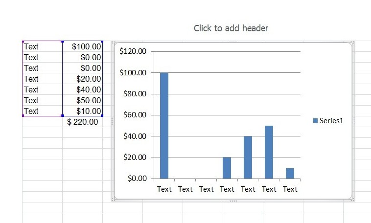
I've searched high and low for this one. Can you help? I don't want to include the $0.00 values when charting this list. Idea?

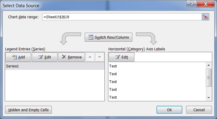
Here a screen shot of the sample list:

Here's the data range. Is this where I edit to get the range to omit a zero value in the list?

 

[GarySmith]

This short video shows that I have a range named "Totals" (and that could be any range, actually) and that we can create a maco (see previous comments) that will hide any zero from the chart with the "Hide Row" function.

A couple of questions now:

1. When we use Hide Row (manually), we must manually "UnHide Row" to get the graph to show the new totals that may have been added to the range (see video).
2. How (if its possible) can we get the column to show "new data", as it's added to the range when it's reference into the "now hidden rows".

Somehow, we'll need to set an "If" statement to show rows in a range, if and when the column in the range has data > 0. Once that happen, the graph will show the visible rows and their values.

Does that make sense?

 

[Piktro]

This short video shows that I have a range named "Totals" (and that could be any range, actually) and that we can create a maco (see previous comments) that will hide any zero from the chart with the "Hide Row" function.

A couple of questions now:

1. When we use Hide Row (manually), we must manually "UnHide Row" to get the graph to show the new totals that may have been added to the range (see video).
2. How (if its possible) can we get the column to show "new data", as it's added to the range when it's reference into the "now hidden rows".

Somehow, we'll need to set an "If" statement to show rows in a range, if and when the column in the range has data > 0. Once that happen, the graph will show the visible rows and their values.

Does that make sense?

I'm definitely not the best person for this, as I'm not super familiar with Macros, but this seems to work. I added an ELSE to the If statement, for cases when the cell does NOT equal 0, it will show the row.

Sub HideRows()
Dim cell As Range
    For Each cell In Range("B1:B7")

If UCase(cell.Value) = "0" Then
    cell.EntireRow.Hidden = True
 Else
    cell.EntireRow.Hidden = False
End If
Next
End Sub

Once you replace your current hide rows macro with this, go to your developer tab and insert a button to regenerate the chart (assign it to the macro).

 

[GarySmith]

I wasn't successful with that solution. hummm...

 

[GarySmith]

Here's a new video that helps explain what I'm trying to achieve (I believe we're almost there).

SEE VIDEO HERE

 

[GarySmith]

Still no idea anyone? See Video Link Above ...

 

[oldbrewer]

you did not reply to my question - I repeat it, if you have 8 data values, and 3 are 0.00, do you want a bar chart with just 5 bars?

 

[GarySmith]

Yes to answer your question about visible bars remaining. Please watch the video above to see that I want a new chart to show the current line totals if changed in the reference page. Maybe that action could be rendered upon worksheet entry?

 

[mmiles19]

I had a similar issue. What I did was add a "Lock Sheet" checkbox, so that after you've entered all your data, you check the box and the sheet with run a "hide rows" macro to hide rows with zeros and then protect the sheet. Then, when you want to change the data, you can uncheck the box which unprotects the sheet and then runs ActiveSheet.Cells.EntireRow.Hidden = False make all rows unhidden again. This will allow it to unhide the rows because it selects every cell in the sheet. However, it may not be very ideal if you plan on having a lot of rows with zeros, which might be kind of overwelming.

 

[GarySmith]

I had a similar issue. What I did was add a "Lock Sheet" checkbox, so that after you've entered all your data, you check the box and the sheet with run a "hide rows" macro to hide rows with zeros and then protect the sheet. Then, when you want to change the data, you can uncheck the box which unprotects the sheet and then runs ActiveSheet.Cells.EntireRow.Hidden = False make all rows unhidden again. This will allow it to unhide the rows because it selects every cell in the sheet. However, it may not be very ideal if you plan on having a lot of rows with zeros, which might be kind of overwelming.

Thanks...I'll give that a try!

 

[oldbrewer]

item	description	number	numberplus
1	text1	5	5.0000001					0	0
2	text2	0	0					0	0
3	text3	9	9.0000003					0	0
4	text4	4	4.0000004					0	0
5	text5	0	0		text4	4.0000004		4	1		text1	5
6	text6	0	0		text7	4.0000007		7	3		text3	9
7	text7	4	4.0000007		text1	5.0000001		1	4		text4	4
8	text8	7	7.0000008		text8	7.0000008		8	7		text7	4
9	text9	0	0		text10	8.000001		10	8		text8	7
10	text10	8	8.000001		text3	9.0000003		3	10		text10	5
	A SERIES OF LOGICAL OPERATIONS SORTS THE DATA UNTIL IT IS IN ORDER BUT AT THE BOTTOM OF THE LAST BLOCK. Selecting all 10 rows AND BOTH COLUMNS of the LAST block and constructing your bar chart will only plot the non blank items as you requested. NO MACROS INVOLVED.

<colgroup><col><col><col><col><col><col><col><col><col><col><col><col><col><col></colgroup><tbody>
</tbody>