Over-ride conditional formatting if adjacent cell is not blank.

[Corinnes]

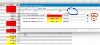
I have set up conditional formatting to highlight dates which are falling due or overdue (THIS MONTH, NEXT MONTH, LAST MONTH).

See sample, Cell F7 has a date entered as it has been sent and so cell E7 no longer needs to be highlighted in pink. The problem I have is that column E has a formula in it already.

How do I get the conditional formatting to not apply (or other words the cell to be shaded in gray) once a date is entered into the adjacent column, and I how do I make this happen for the whole column?

Thanks in advance.

 

[Anthony47]

You need to add to your current confitional format formula le conditiona that column F is empty. Example:
-select E3:E1000
-assign a conditional format using the formula =AND(YourCurrentFormula,$F6="")

 

[Corinnes]

You need to add to your current confitional format formula le conditiona that column F is empty. Example:
-select E3:E1000
-assign a conditional format using the formula =AND(YourCurrentFormula,$F6="" [/QUOTE] [QUOTE="Anthony47, post: 6046870, member: 60147"] )

Thank you for responding. I am currently using the 'Format only cells that contain' conditional formatting and not a formula so I may need to change this to a combined formula?

 

[Anthony47]

Yes, you need to set your C.F. "using a formula". Thus
-select E2:E1000 (or a range more suitable, but start from E2 and avoind using a whole column
-set 3 CF using the following formulas + Color:

=AND($E2<EOMONTH(TODAY(),-1),$F2="")                    Color RED, last month (or older)

=AND($E2<EOMONTH(TODAY(),0),$F2="")                      Color Orange, this month

=AND($E2<EOMONTH(TODAY(),1),$F2="")                      Color Yellow, next month

With reference to the attached image
a) use the "arrows" circled in blue to set the hierarchy of the rules as shows (select a rule, use the arrows to move the rule higher or lower in the sequence)
b) use the checkbox circled in red to stop other rules to be evaluated, if rule is true

Try...

 

[Corinnes]

Brilliant! This worked. Thank you kindly.

 

[Anthony47]

Thank you for the feedback
If that resolve the problem then it'd be better to mark the discussion as Resoved; see the procedure: Mark as Solution