Payment term and Cash flow (formula linked with costs)

Adfinance

Board Regular
Joined
Jan 1, 2021
Messages
80
Office Version
  1. 365
Platform
  1. Windows
Hi everyone, I need to calculate automatically the cash position (cashout) based on payment terms and costs.
The payment terms may change, so I need a dynamic formula.
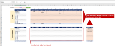
Attached you will see that there is a section with "P&L impact", with the listing of all the costs and their value month by month (if any).

Also, you will see in the "Cash flow impact" section that I need to find a formula (in cells S19 to Q28) which depends on 2 things:
1/ Cost value (from cells F5 to Q14)
2/ Payment term in days (cells S19 to S28)

For instance, if I put the value 8000 in cell F5, and Payment term in cell S19 is 40 days, thanks to the formula we will have automatically the value 8000 in cell G19.

Can anyone help me please?
 

Attachments

  • Excel issue.PNG
    Excel issue.PNG
    51.6 KB · Views: 670

Excel Facts

Format cells as time
Select range and press Ctrl+Shift+2 to format cells as time. (Shift 2 is the @ sign).
Welcome to MrExcel Message Board.
Please give more examples and upload your file with XL2BB ADDIN (preferable) or at Free hosting site and then input link here. e.g. www.dropbox.com
Examples if your Payment less than 40 result is 8000 and ....
Are Result different for each month.
Is your starting date is 1/1/2021.
and ....
 
Upvote 0
Hi maabadi.
Example, if for your first expense you have a cost of 8000 in January 2021, and a payment term of 40 days, it means that you will have a cashout (in the second table) of 8000 as well (but in February, not in January ... so the value will be automatically displayed in January because it's a payment term of 40 days).

With the same example, if the payment term was 200 days, the value "8000" in january 2021 (in the P&L section, for costs) would have been displayed in july 2021 for the cash outflow.
The same is the payment term is less than 40 days (let's say : 23 days), the cash outflow would be in the same month (here in January). If the payment term exceeds the number of days for the month (for instance, january you have a total of 31 days), then the cash out will be displayed in February, not in January.
 
Upvote 0
And What about if your payment Day is in less than of month that displayed First Value. For Example if payment if less than 40 days and first Value is in March , Minimum 60 days,Are Value comes in March or Feb. (row 2 & 3 of your Data).
And Please upload Example file.
 
Upvote 0
Try This:
Redditexcel.xlsx
CDEFGHIJKLMNOPQRS
1
2Start Date1/1/2021
3
4Nature of ExpenseJan-21Feb-21Mar-21Apr-21May-21Jun-21Jul-21Aug-21Sep-21Oct-21Nov-21Dec-21
5Expense No. 18,000-----------
6Expense No. 2--4,000---------
7Expense No. 3-----500------
8
9
10
11
12
13
14
15SubTotal8,000-4,000--500------
16
17
18Nature of ExpenseJan-21Feb-21Mar-21Apr-21May-21Jun-21Jul-21Aug-21Sep-21Oct-21Nov-21Dec-21Payment Terms(s)
19Expense No. 1-8,000----------+ 40 Day(s)
20Expense No. 2--4,000---------+ 15 Day(s)
21Expense No. 3-----------500+ 200 Day(s)
22------------
23------------
24------------
25------------
26------------
27------------
28------------
29SubTotal-8,0004,000--------500
30
Sheet1
Cell Formulas
RangeFormula
F15F15=SUBTOTAL(109,[Jan-21])
G15G15=SUBTOTAL(109,[Feb-21])
H15H15=SUBTOTAL(109,[Mar-21])
I15I15=SUBTOTAL(109,[Apr-21])
J15J15=SUBTOTAL(109,[May-21])
K15K15=SUBTOTAL(109,[Jun-21])
L15L15=SUBTOTAL(109,[Jul-21])
M15M15=SUBTOTAL(109,[Aug-21])
N15N15=SUBTOTAL(109,[Sep-21])
O15O15=SUBTOTAL(109,[Oct-21])
P15P15=SUBTOTAL(109,[Nov-21])
Q15Q15=SUBTOTAL(109,[Dec-21])
G18:Q18G18=EOMONTH(F18,0)+1
F19:Q28F19=IF(SUM($F5:F5)=0,0,IF(AND(F$18-INDEX($F$18:$Q$18,1,MATCH( 0,$F5:$Q5,-1))<$S19,EOMONTH(F$18,0)-INDEX($F$18:$Q$18,1,MATCH( 0,$F5:$Q5,-1))>$S19),SUM($F5:F5),0))
F29F29=SUBTOTAL(109,Sheet1!$F$19:$F$28)
G29G29=SUBTOTAL(109,Sheet1!$G$19:$G$28)
H29H29=SUBTOTAL(109,Sheet1!$H$19:$H$28)
I29I29=SUBTOTAL(109,Sheet1!$I$19:$I$28)
J29J29=SUBTOTAL(109,Sheet1!$J$19:$J$28)
K29K29=SUBTOTAL(109,Sheet1!$K$19:$K$28)
L29L29=SUBTOTAL(109,Sheet1!$L$19:$L$28)
M29M29=SUBTOTAL(109,Sheet1!$M$19:$M$28)
N29N29=SUBTOTAL(109,Sheet1!$N$19:$N$28)
O29O29=SUBTOTAL(109,Sheet1!$O$19:$O$28)
P29P29=SUBTOTAL(109,Sheet1!$P$19:$P$28)
Q29Q29=SUBTOTAL(109,Sheet1!$Q$19:$Q$28)
 
Upvote 0
Hi maabadi, could you please send me your email? I will send you the file there, because it does not work here unfortunately.

Regardind the formula, the idea is to have pretty much the "same" formula everywhere in the below table .... and if I decide to change many times one or several Payment terms (just to see the outcome), or one of several costs values, the table with the cash has to change accordingy (and automatically).
Thus, the formulas with a "sumtotal" won't work. Because if in cell S19 (payment term for the all the values for cost n°1 (from F5 to Q5)) I decide to put let's say 200 days instead of the actual value which is 40 days .... then if we have:
a) 8 000 in cell F5 (with payment term term of 200 days: cell S19)
b) 10 000 in cell K5 (with payment term term of 200 days: cell S19)

The value 8 000 (with the correct formula) will be displayed automatically in the cell L19 ... for the cash flow impact
The value 10 000 (with the correct formula) will be displayed automatically in the cell Q19 ... for the cash flow impact

Note that: Cost values are added manually and they could be different each month if wanted. Each cost value is displayed "once" in the "cash flow impacct Table". We could have many cost values for Expense n°1 (for instance one in January, one in February, one in July, etc.)

The same for each Expense from line 5 to 14.
 
Upvote 0
In your different cells formulas, the only formula I am looking for here is you formula in cell F19 (that I will copy past in all the table as wellfrom cell F19 to Q28).
Unfortunately you formula in F19 does not work. Please send me your email so that I can share with you my file.
 
Upvote 0

Forum statistics

Threads
1,214,611
Messages
6,120,510
Members
448,967
Latest member
screechyboy79

We've detected that you are using an adblocker.

We have a great community of people providing Excel help here, but the hosting costs are enormous. You can help keep this site running by allowing ads on MrExcel.com.
Allow Ads at MrExcel

Which adblocker are you using?

Disable AdBlock

Follow these easy steps to disable AdBlock

1)Click on the icon in the browser’s toolbar.
2)Click on the icon in the browser’s toolbar.
2)Click on the "Pause on this site" option.
Go back

Disable AdBlock Plus

Follow these easy steps to disable AdBlock Plus

1)Click on the icon in the browser’s toolbar.
2)Click on the toggle to disable it for "mrexcel.com".
Go back

Disable uBlock Origin

Follow these easy steps to disable uBlock Origin

1)Click on the icon in the browser’s toolbar.
2)Click on the "Power" button.
3)Click on the "Refresh" button.
Go back

Disable uBlock

Follow these easy steps to disable uBlock

1)Click on the icon in the browser’s toolbar.
2)Click on the "Power" button.
3)Click on the "Refresh" button.
Go back
Back
Top