Payment term and Cash flow (formula linked with costs)

Adfinance

Board Regular
Joined
Jan 1, 2021
Messages
80
Office Version
  1. 365
Platform
  1. Windows
Hi everyone, I need to calculate automatically the cash position (cashout) based on payment terms and costs.
The payment terms may change, so I need a dynamic formula.
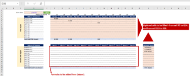
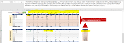
Attached you will see that there is a section with "P&L impact", with the listing of all the costs and their value month by month (if any).

Also, you will see in the "Cash flow impact" section that I need to find a formula (in cells S19 to Q28) which depends on 2 things:
1/ Cost value (from cells F5 to Q14)
2/ Payment term in days (cells S19 to S28)

For instance, if I put the value 8000 in cell F5, and Payment term in cell S19 is 40 days, thanks to the formula we will have automatically the value 8000 in cell G19.

Can anyone help me please?
 

Attachments

  • Excel issue.PNG
    Excel issue.PNG
    51.6 KB · Views: 676
Hi @maabadi thank you very much. Unfortunately when I insert the formula in my excel file, it does not work (mayne a problem of "coma" or something like that?).

It seems to be perfectly working with your example above ... or maybe could you just send me your file with the formula (directly in the sheet, to be sure it works)? Thank you so much again.
You can access the file with your last formula here: For Mr Excel error formula v2.xlsx

I don't know why it's not working there .. could you help with that? Thanks again!
 
Upvote 0

Excel Facts

Move date out one month or year
Use =EDATE(A2,1) for one month later. Use EDATE(A2,12) for one year later.
You Imported Dash Not Zero At your first Table and you should replace all "-" with zero, then change number format to
_(* #,##0_);_(* (#,##0);_(* "-"??_);_(@_)
 
Upvote 0
Please Change "-" with Zero at your first tabel. AND I forgot to Add = to 2 part of formula. This is modified version:
Excel Formula:
=IFERROR(IF(SUM($F5:F5)=0,0,IF(AND(INDEX($F$4:$Q$4,,MATCH(TRUE,INDEX($F5:$Q5>0,0),0))+$S19>F$18,INDEX($F$4:$Q$4,,MATCH(TRUE,INDEX($F5:$Q5>0,0),0))+$S19<=EOMONTH(F$18,0)),INDEX($F5:$Q5,,MATCH(TRUE,INDEX($F5:$Q5>0,0),0)),IF(INDEX($F$4:$Q$4,,MATCH(TRUE,INDEX($F5:$Q5>0,0),0))+$S19>=F$18,0,INDEX($F5:$Q5,,MATCH(TRUE,INDEX($F5:$Q5>0,0),0)+COLUMNS($F19:F19)+1-IFERROR(MATCH(TRUE,INDEX($E19:E19>0,0),0),1))))),"")
Thank you very much. Now it works, BUT still we have a last issue. I will clarify ...
January 2021 we have: 31 days (line 3 of the sheet)
January 2021 + February 2021 we have: 59 days (line 3 of the sheet)
January 2021 + February 2021 + March 2021 we have: 90 days (line 3 of the sheet)
etc. until january to december 2021 where we have in total 365 days.

If in "Payment terms" I decide to put for instance 31 days or 59 days or 90 days or 365 days etc (the errors will be with the exact sum of days for the months) then it won't work. You can test it in the excel file to see.

Do you know what do I have to change in your last formula to change it?

For example, if we put 151 days in the cell S19, it means it will be the last day of May for the value " 5000" in cell F5. So at the end we will have this value displayed in cell J19. And so on.
Again, thank you so much!
 
Last edited:
Upvote 0
I think this is What you want:
Excel Formula:
=IFERROR(IF(SUM($F5:F5)=0,0,IF(AND(INDEX($F$4:$Q$4,,MATCH(TRUE,INDEX($F5:$Q5>0,0),0))+$S19>=F$18,INDEX($F$4:$Q$4,,MATCH(TRUE,INDEX($F5:$Q5>0,0),0))+$S19<=EOMONTH(F$18,0)),INDEX($F5:$Q5,,MATCH(TRUE,INDEX($F5:$Q5>0,0),0)),IF(INDEX($F$4:$Q$4,,MATCH(TRUE,INDEX($F5:$Q5>0,0),0))+$S19>=F$18,0,INDEX($F5:$Q5,,MATCH(TRUE,INDEX($F5:$Q5>0,0),0)+COLUMNS($F19:F19)+1-IFERROR(MATCH(TRUE,INDEX($E19:E19>0,0),0),1))))),"")
Not exactly ... your new formula does not work (please see attached).
2 issues:
> First issue is that the formula does not work in all the cells
> Second issue is that let's say I put 151 days in "Payment term" (cell S19). So, 151 days corresponds to the last day of May (look at the values in line 2 of the attached file to understand better).

Sorry to ask again, but do you have the solution?

Thank you so much!
 

Attachments

  • 1609688859790.png
    1609688859790.png
    119.8 KB · Views: 18
Upvote 0
Not exactly ... your new formula does not work (please see attached).
2 issues:
> First issue is that the formula does not work in all the cells
> Second issue is that let's say I put 151 days in "Payment term" (cell S19). So, 151 days corresponds to the last day of May (look at the values in line 2 of the attached file to understand better).

Sorry to ask again, but do you have the solution?

Thank you so much!
@maabadi :)
 
Upvote 0
For me working at all cells. Check again all value of Zero.
and I think you count the day on it then 1+151 = 152 and formula works correct if you don't count the first day use this:
Excel Formula:
=IFERROR(IF(SUM($F5:F5)=0,0,IF(AND(INDEX($F$4:$Q$4,,MATCH(TRUE,INDEX($F5:$Q5>0,0),0))+$S19>=F$18+1,INDEX($F$4:$Q$4,,MATCH(TRUE,INDEX($F5:$Q5>0,0),0))+$S19-1<=EOMONTH(F$18,0)),INDEX($F5:$Q5,,MATCH(TRUE,INDEX($F5:$Q5>0,0),0)),IF(INDEX($F$4:$Q$4,,MATCH(TRUE,INDEX($F5:$Q5>0,0),0))+$S19>=F$18+1,0,INDEX($F5:$Q5,,MATCH(TRUE,INDEX($F5:$Q5>0,0),0)+COLUMNS($F19:F19)+1-IFERROR(MATCH(TRUE,INDEX($E19:E19>0,0),0),1))))),"")
It's finally working :) Thank you so much, you're definitely an expert! Looking forward to working with you again in the future! @maabadi
 
Upvote 0

Forum statistics

Threads
1,214,972
Messages
6,122,530
Members
449,088
Latest member
RandomExceller01

We've detected that you are using an adblocker.

We have a great community of people providing Excel help here, but the hosting costs are enormous. You can help keep this site running by allowing ads on MrExcel.com.
Allow Ads at MrExcel

Which adblocker are you using?

Disable AdBlock

Follow these easy steps to disable AdBlock

1)Click on the icon in the browser’s toolbar.
2)Click on the icon in the browser’s toolbar.
2)Click on the "Pause on this site" option.
Go back

Disable AdBlock Plus

Follow these easy steps to disable AdBlock Plus

1)Click on the icon in the browser’s toolbar.
2)Click on the toggle to disable it for "mrexcel.com".
Go back

Disable uBlock Origin

Follow these easy steps to disable uBlock Origin

1)Click on the icon in the browser’s toolbar.
2)Click on the "Power" button.
3)Click on the "Refresh" button.
Go back

Disable uBlock

Follow these easy steps to disable uBlock

1)Click on the icon in the browser’s toolbar.
2)Click on the "Power" button.
3)Click on the "Refresh" button.
Go back
Back
Top