Payment terms (formula) for P&L impact and Cash flow

[Adfinance]

Hi everyone, how are you?
Could I ask you to help me please?

I need to calculate automatically 2 things (see the link below - in the tab "Cost details"):
1/ The P&L impact (taking into account several variables - from cell L13 to cell S13
2/ the Cash position (cashout) based on payment terms, total cost expense, start month and date, etc.. The payment terms may change (from cell D28 to cell D37), so I need dynamic formulas.
Can anyone help me please?

All the details to help you are displayed in the Excel file, in the tab "Instructions". And your outcome will be in the tab "Cost details".
Thank you soooo much for your help, it would be really helpful to me.

Link to access the excel file here:

To send to Mr Excel - version 1.xlsx

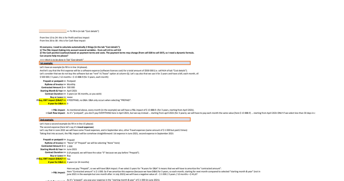
Instructions >> To fill in (in tab "Cost details") From line 13 to 24: this is for Profit and loss impact From line 26 to 38 : this is for Cash flow impact Hi everyone, I need to calculate automatically 2 things (in the tab "Cost details"): 1/ The P&L impact (taking into account several variabl...

docs.google.com

@maabadi

 

[maabadi]

I told before, I have many works these days to do & take time to answer to you.
1. At Cost Detail Sheet. Correct Formula to This at Cell Y14 and then Drag it right & down.

=IF($D14="OPEX",SUM(OFFSET($AJ14,0,(COLUMNS($Y:Y)-1)*12,1,12)),IF(AND(SUM(OFFSET($AJ14,0,(COLUMNS($Y:Y)-1)*12,1,12))<>0,SUM($X14:X14)=0),INDEX(OFFSET($AJ14,0,(COLUMNS($Y:Y)-1)*12,1,12),MATCH(TRUE,INDEX((OFFSET($AJ14,0,(COLUMNS($Y:Y)-1)*12,1,12)<0),0),0)),0))

after adding this formula you can see wanted results at Executive Summary Sheet.
Otherwise if you want previous data & values, use this one formula at all range:

=SUM(OFFSET($AJ14,0,(COLUMNS($Y:Y)-1)*12,1,12))

2. if you don't want First part, you should use it at another place and then from them you can see correct results at Executive Summary Sheet.

 

[Adfinance]

I told before, I have many works these days to do & take time to answer to you.
1. At Cost Detail Sheet. Correct Formula to This at Cell Y14 and then Drag it right & down.

=IF($D14="OPEX",SUM(OFFSET($AJ14,0,(COLUMNS($Y:Y)-1)*12,1,12)),IF(AND(SUM(OFFSET($AJ14,0,(COLUMNS($Y:Y)-1)*12,1,12))<>0,SUM($X14:X14)=0),INDEX(OFFSET($AJ14,0,(COLUMNS($Y:Y)-1)*12,1,12),MATCH(TRUE,INDEX((OFFSET($AJ14,0,(COLUMNS($Y:Y)-1)*12,1,12)<0),0),0)),0))

after adding this formula you can see wanted results at Executive Summary Sheet.
Otherwise if you want previous data & values, use this one formula at all range:

=SUM(OFFSET($AJ14,0,(COLUMNS($Y:Y)-1)*12,1,12))

2. if you don't want First part, you should use it at another place and then from them you can see correct results at Executive Summary Sheet.

 

[Adfinance]

Thank you @maabadi

Actually (based on what has been share at post #80 ... we won't use the "Capex" or "Opex" selection at column D from tab "Cost details" ... I mean for the formula ... do you think it's possible?

Note that the formula won't be based on column D from tab "Cost details" ... But it will be based on other inputs: "BUY" or "LEASE", etc.
We do not have CAPEX or OPEX notions in the formulas, but based on post #80 we know how to classify thing in CAPEX and OPEX (in tab "Executive summary" I mean)

The actual formula is wrong. Please, the formulas to be modified are only those in tab "Executive summary", at line 28 & 30 & 33 & 35.
Do tell if there is something unclear. Thank you so much.

 

[maabadi]

This is complex. Please ask it as new thread.
You want sum of first values at Y14 to AU23 for CAPEX & you want sum of all values at Y14 to AU23 for APEX.

 

[Adfinance]

This is complex. Please ask it as new thread.
You want sum of first values at Y14 to AU23 for CAPEX & you want sum of all values at Y14 to AU23 for APEX.

Atually it depends.

If we choose "BUY", then yes, the first value on the left side of the line will be for CAPEX, and all the other values of the line will be for OPEX
If we choose "LEASE", then ALL the values from the line here will be for OPEX.

Is it something you can do? Formulas to be put only in tab "Executive summary", at lines 28 & 30 & 33 & 35.
But the formula will be taking into account values in "Cost details" tab only (for "Software" section ... line 14 to 23 / for "Infrastructure" section ... line 44 to 53)

Is it something you can do?

Please let's stay in this thread (it's only this formula and then it's done )
Thank you so much @maabadi !

 

[maabadi]

I can do it for one row but for sum of that values at row 14 -23 , I have problem.
Please ask as new thread with only one example file with random data to see others recommendations. Then we can take better options.
Also I have works these days and very low time to think & work on it.

 

[Adfinance]

I can do it for one row but for sum of that values at row 14 -23 , I have problem.
Please ask as new thread with only one example file with random data to see others recommendations. Then we can take better options.
Also I have works these days and very low time to think & work on it.

Maybe we could create another intermediary "tab" for that? In this new tab we would have:
(i) a part of the values for CAPEX results
(ii) a part of the values for OPEX results
... and then base the final formulas of the tab "Exec summary" on this new sheet with these values??

Do you think it would be the best way? And then I will hide this tab at the end ..

Thank you @maabadi

 

[maabadi]

A. you can also change formula at Y28 to this. then drag it Right & down to AH37.
1. if your month at AJ13 always start with January:

=sum(offset($AJ28,0,(Columns($Y:Y) - 1)*12,1,12))

2. if Month at AJ13 Change with time ( if you see Error Try it With Press CTRL+SHIFT+ENTER). it show error on google sheet but for me work on excel:

=SUMPRODUCT(($AJ28:$EY28),(--($AJ28:$EY28<>""))*(YEAR($AJ$13:$EY$13)=YEAR($AJ$13)-1+COLUMNS($Y:Y)))

B. Other formula I add at FormulaAssumptions Sheet.
1. From G27 to P38 for OPEX
I add formula to your file if see error test it on excel file. this is formula at G27:

=IF(SUM($R28:$AA28)=0,IF('Cost details'!Y28=0,"",'Cost details'!Y28),"")

2. From R27 to AA38 for CAPEX
I add formula to your file if see error test it on excel file. this is formula at R27 (Press CTRL+SHIFT+ENTER):

=IFNA(INDEX('Cost details'!$AJ28:$EY28,,MATCH(1,(YEAR('Cost details'!$AJ$13:$EY$13)=R$27)*('Cost details'!$AJ28:$EY28='Cost details'!$N14*-1)*('Cost details'!$R14="BUY"),0)),"")

Then Drag both down.

3. at rows 38 I Sum total values that Can you use it Executive summary tab I think.
For Example at G38:

=SUM(G28:G37)

 

[Adfinance]

A. you can also change formula at Y28 to this. then drag it Right & down to AH37.
1. if your month at AJ13 always start with January:

=sum(offset($AJ28,0,(Columns($Y:Y) - 1)*12,1,12))

2. if Month at AJ13 Change with time ( if you see Error Try it With Press CTRL+SHIFT+ENTER). it show error on google sheet but for me work on excel:

=SUMPRODUCT(($AJ28:$EY28),(--($AJ28:$EY28<>""))*(YEAR($AJ$13:$EY$13)=YEAR($AJ$13)-1+COLUMNS($Y:Y)))

B. Other formula I add at FormulaAssumptions Sheet.
1. From G27 to P38 for OPEX
I add formula to your file if see error test it on excel file. this is formula at G27:

=IF(SUM($R28:$AA28)=0,IF('Cost details'!Y28=0,"",'Cost details'!Y28),"")

2. From R27 to AA38 for CAPEX
I add formula to your file if see error test it on excel file. this is formula at R27 (Press CTRL+SHIFT+ENTER):

=IFNA(INDEX('Cost details'!$AJ28:$EY28,,MATCH(1,(YEAR('Cost details'!$AJ$13:$EY$13)=R$27)*('Cost details'!$AJ28:$EY28='Cost details'!$N14*-1)*('Cost details'!$R14="BUY"),0)),"")

Then Drag both down.

3. at rows 38 I Sum total values that Can you use it Executive summary tab I think.
For Example at G38:

=SUM(G28:G37)

Hi @maabadi it does not work. I will give you my feedback soon

 

[Adfinance]

Hi @maabadi it does not work. I will give you my feedback soon

Hi @maabadi
New file (with an update on tab "CapexOpex" only):

https://docs.google.com/spreadsheets/d/1vxctUdSiMluwvK5UTTgDMcXRVnEjbh2A/edit?usp=drive_web&ouid=114111419884827392378&rtpof=true

Maybe could you just please try this at tab "CapexOpex" only (do not touch the "Executive summary" tab, only work on "CapexOpex" tab, and then I will adjust myself on the tab "Executive summary". The formula will be based on either "BUY" selection or "LEASE" selection.

I - First formula to be put at tab "CapexOpex", from cell P7 to EE17:
> This is for "Capex - Software" at tab "Executive summary", line 28
1/ Let's begin with the formula from P7 to EE7 (same line) then drag and drop.
If "BUY" selection at cell R14 (tab "Cost details"), then the values displayed in "CapexOpex" tab (line 7) will be the following:
The total value from "total contracted amount" (which is the first value on the left side at tab "Cost details", from cell AJ14 to EY14) will be displayed at line 7 tab "CapexOpex" (from cell P7 to EE7).

NOTE THAT THE VALUES RELATED TO "EBIT IMPACT" WILL NOT BE DISPLAYED IN "CAPEX". BUT HERE IN THE EXAMPLE WITH "BUY" IT WILL BE DISPLAYED IN "OPEX" (line 21 in tab "CapexOpex")

The values that are related to "EBIT impact" will be (in this example wih "BUY" selection) all the values after the first one on the left.

The value(s) from the "total contracted amount" are here considered as CAPEX (if "BUY" selection) or are considered as OPEX (if "LEASE selection")
And ... the values from EBIT impact are considered as OPEX (always, no matter what .... it could be "BUY" or "LEASE" ... always OPEX).

Please try to have the right formula at line 7 (from P7 to EE7) of tab "CapexOpex", then we will drag and drop".


Thank you so much @maabadi you are a life savior