Ideally you want to address this at the source, it is unlikely that the data comes this way without it being manipulated. Get them to give it to you in its more natural state.
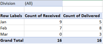
Its pretty easy to convert this using Power Query. Either in a summarised form or if you "Unpivot" it, it would become Pivot Table Friendly.
Alternatively you could just use formulas.
The formulas are already there, I called the Table "tblData"
If either of the Power Query options are of interest, I can give you either the code or the steps to get there, just let me know.
| 20210528 Transpose for Chart.xlsx |
|---|
|
|---|
| A | B | C | D | E | F | G | H | I | J | K | L | M | N | O | P | Q |
|---|
| 1 | | | | | | | | | | | | | | | | | |
|---|
| 2 | | Original Data | | | | Formula Version | | | | | | | | | | | |
|---|
| 3 | | | | | | | | | | | | | | | | | |
|---|
| 4 | | Division | Received | Delivered | | | Jan | Feb | Mar | Apr | May | | | | | | |
|---|
| 5 | | A | Jan | Jan | | Received | 9 | 7 | 0 | 0 | 0 | | | | | | |
|---|
| 6 | | A | Jan | Jan | | Delivered | 5 | 9 | 2 | 0 | 0 | | | | | | |
|---|
| 7 | | A | Jan | Jan | | | | | | | | | | | | | |
|---|
| 8 | | A | Jan | Feb | | Power Query Summary Version | | | | | | | | | | | |
|---|
| 9 | | A | Jan | Feb | | | | | | | | | | | | | |
|---|
| 10 | | A | Feb | Feb | | Attribute | Jan | Feb | Mar | | | | | | | | |
|---|
| 11 | | B | Jan | Jan | | Received | 9 | 7 | 0 | | | | | | | | |
|---|
| 12 | | B | Jan | Jan | | Delivered | 5 | 9 | 2 | | | | | | | | |
|---|
| 13 | | B | Feb | Feb | | | | | | | | | | | | | |
|---|
| 14 | | B | Feb | Feb | | | | | | | | | | | | | |
|---|
| 15 | | B | Feb | Mar | | | | | | | | | | | | | |
|---|
| 16 | | C | Jan | Feb | | | | | | | | | | | | | |
|---|
| 17 | | C | Jan | Feb | | Power Query Unpivot Version | | | | | Pivot Based on Unpivot PQ | | | | | | |
|---|
| 18 | | C | Feb | Feb | | | | | | | | | | | | | |
|---|
| 19 | | C | Feb | Feb | | Division | Status | Month | | | Count of Status | | Month | | | | |
|---|
| 20 | | C | Feb | Mar | | A | Received | Jan | | | Status | Division | Jan | Feb | Mar | Grand Total | |
|---|
| 21 | | | | | | A | Delivered | Jan | | | Delivered | A | 3 | 3 | | 6 | |
|---|
| 22 | | | | | | A | Received | Jan | | | | B | 2 | 2 | 1 | 5 | |
|---|
| 23 | | | | | | A | Delivered | Jan | | | | C | | 4 | 1 | 5 | |
|---|
| 24 | | | | | | A | Received | Jan | | | Delivered Total | | 5 | 9 | 2 | 16 | |
|---|
| 25 | | | | | | A | Delivered | Jan | | | Received | A | 5 | 1 | | 6 | |
|---|
| 26 | | | | | | A | Received | Jan | | | | B | 2 | 3 | | 5 | |
|---|
| 27 | | | | | | A | Delivered | Feb | | | | C | 2 | 3 | | 5 | |
|---|
| 28 | | | | | | A | Received | Jan | | | Received Total | | 9 | 7 | | 16 | |
|---|
| 29 | | | | | | A | Delivered | Feb | | | Grand Total | | 14 | 16 | 2 | 32 | |
|---|
| 30 | | | | | | A | Received | Feb | | | | | | | | | |
|---|
| 31 | | | | | | A | Delivered | Feb | | | | | | | | | |
|---|
| 32 | | | | | | B | Received | Jan | | | | | | | | | |
|---|
| 33 | | | | | | B | Delivered | Jan | | | | | | | | | |
|---|
| 34 | | | | | | B | Received | Jan | | | | | | | | | |
|---|
| 35 | | | | | | B | Delivered | Jan | | | | | | | | | |
|---|
| 36 | | | | | | B | Received | Feb | | | | | | | | | |
|---|
| 37 | | | | | | B | Delivered | Feb | | | | | | | | | |
|---|
| 38 | | | | | | B | Received | Feb | | | | | | | | | |
|---|
| 39 | | | | | | B | Delivered | Feb | | | | | | | | | |
|---|
| 40 | | | | | | B | Received | Feb | | | | | | | | | |
|---|
| 41 | | | | | | B | Delivered | Mar | | | | | | | | | |
|---|
| 42 | | | | | | C | Received | Jan | | | | | | | | | |
|---|
| 43 | | | | | | C | Delivered | Feb | | | | | | | | | |
|---|
| 44 | | | | | | C | Received | Jan | | | | | | | | | |
|---|
| 45 | | | | | | C | Delivered | Feb | | | | | | | | | |
|---|
| 46 | | | | | | C | Received | Feb | | | | | | | | | |
|---|
| 47 | | | | | | C | Delivered | Feb | | | | | | | | | |
|---|
| 48 | | | | | | C | Received | Feb | | | | | | | | | |
|---|
| 49 | | | | | | C | Delivered | Feb | | | | | | | | | |
|---|
| 50 | | | | | | C | Received | Feb | | | | | | | | | |
|---|
| 51 | | | | | | C | Delivered | Mar | | | | | | | | | |
|---|
| 52 | | | | | | | | | | | | | | | | | |
|---|
|
|---|