Polynomial function

[Duane]

Hey gang.

Excel can give us linear, exponential and polynomial trendlines.

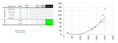
To forecast unknown Ys based on known Xs, I've used

• for linear, =ROUND(FORECAST and the plot points perfectly land where Excel would have put them by adding a linear trendline
• for Exponential =GROWTH, and the plot points perfectly land where Excel would have put them by adding an exponential trendline (both for true and false)
• for polynomial (order 2), ...??

What formula can I use to give me the plot points that land under the trendline that Excel provides by adding the polynomial order 2 trendline?

 

[KRice]

I'm not quite sure that I understand what you want. If you perform a 2nd order regression, you can extract the coefficients of the curve as shown here and then use them to determine any set of (Xreg,Yreg) points on the regression curve.

MrExcel20210209.xlsx
	B	C	D
1	X	Y
2	237	8
3	1716	29
4	1910	38
5	2250	65
6
7
8
9	2nd order regression
10	x2	x	b
11	2.73624E-05	-0.03997	15.96755
12
13	Xreg	Yreg
14	500	2.824295
15	1000	3.362224
16	1500	17.58134
17	2000	45.48163
Duane

Cell Formulas
Range	Formula
B11:D11	B11	=LINEST(C2:C5,B2:B5^{1,2},1,0)
C14:C17	C14	=$B$11*B14^2+$C$11*B14+$D$11
Press CTRL+SHIFT+ENTER to enter array formulas surrounded with curly braces.

 

[Duane]

Hey, thanks for your help.

So, what I'm looking for is, if you look at my column of known Xs and known Ys, you'll see I have known Xs of 2,390 and ,2530 - based on the known Ys from 8 to 65, I used FORECAST to do that for the linear (in yellow); and GROWTH for the Exponential (in green and red), but I need to know what formula will give me the Ys will be for X=2390 and X=2530 based on a polynomial forecast formula. (the green-shaded cells).

 

[KRice]

Have a look at this...based on my previous post, the LINEST function will return the coefficients. But you can leave those coefficients in an array and multiply them by another array containing {x^2, x^1, x^0} and then sum using the SUMPRODUCT function. See the blue input cells and the resulting green output cells. The yellow table shows another less compact approach.

MrExcel20210209.xlsx
	B	C	D
1	X	Y
2	237	8
3	1716	29
4	1910	38
5	2250	65
6	2390	76.7413393
7	2530	89.9930603
8
9	2nd order regression
10	x2	x	b
11	2.73624E-05	-0.0399677	15.96755
12
13	Xreg	Yreg
14	500	2.82429475
15	1000	3.36222418
16	1500	17.5813365
17	2000	45.4816318
18	2390	76.7413393
19	2530	89.9930603
Duane

Cell Formulas
Range	Formula
C6:C7	C6	=SUMPRODUCT(LINEST($C$2:$C$5,$B$2:$B$5^{1,2},1,0)*(B6^{2,1,0}))
B11:D11	B11	=LINEST(C2:C5,B2:B5^{1,2},1,0)
C14:C19	C14	=$B$11*B14^2+$C$11*B14+$D$11
Press CTRL+SHIFT+ENTER to enter array formulas surrounded with curly braces.

 

[Duane]

Have a look at this...based on my previous post, the LINEST function will return the coefficients. But you can leave those coefficients in an array and multiply them by another array containing {x^2, x^1, x^0} and then sum using the SUMPRODUCT function. See the blue input cells and the resulting green output cells. The yellow table shows another less compact approach.

MrExcel20210209.xlsx
	B	C	D
1	X	Y
2	237	8
3	1716	29
4	1910	38
5	2250	65
6	2390	76.7413393
7	2530	89.9930603
8
9	2nd order regression
10	x2	x	b
11	2.73624E-05	-0.0399677	15.96755
12
13	Xreg	Yreg
14	500	2.82429475
15	1000	3.36222418
16	1500	17.5813365
17	2000	45.4816318
18	2390	76.7413393
19	2530	89.9930603
Duane

Cell Formulas
Range	Formula
C6:C7	C6	=SUMPRODUCT(LINEST($C$2:$C$5,$B$2:$B$5^{1,2},1,0)*(B6^{2,1,0}))
B11:D11	B11	=LINEST(C2:C5,B2:B5^{1,2},1,0)
C14:C19	C14	=$B$11*B14^2+$C$11*B14+$D$11
Press CTRL+SHIFT+ENTER to enter array formulas surrounded with curly braces.

That's it! THANK YOU!!!

 

[Duane]

Have a look at this...based on my previous post, the LINEST function will return the coefficients. But you can leave those coefficients in an array and multiply them by another array containing {x^2, x^1, x^0} and then sum using the SUMPRODUCT function. See the blue input cells and the resulting green output cells. The yellow table shows another less compact approach.

MrExcel20210209.xlsx
	B	C	D
1	X	Y
2	237	8
3	1716	29
4	1910	38
5	2250	65
6	2390	76.7413393
7	2530	89.9930603
8
9	2nd order regression
10	x2	x	b
11	2.73624E-05	-0.0399677	15.96755
12
13	Xreg	Yreg
14	500	2.82429475
15	1000	3.36222418
16	1500	17.5813365
17	2000	45.4816318
18	2390	76.7413393
19	2530	89.9930603
Duane

Cell Formulas
Range	Formula
C6:C7	C6	=SUMPRODUCT(LINEST($C$2:$C$5,$B$2:$B$5^{1,2},1,0)*(B6^{2,1,0}))
B11:D11	B11	=LINEST(C2:C5,B2:B5^{1,2},1,0)
C14:C19	C14	=$B$11*B14^2+$C$11*B14+$D$11
Press CTRL+SHIFT+ENTER to enter array formulas surrounded with curly braces.

I needed the formula you provided in C6:C7, thanks much!

The conversation may continue to further explore the formulas in B11:D11...please stay tuned...

 

[Duane]

I needed the formula you provided in C6:C7, thanks much!

The conversation may continue to further explore the formulas in B11:D11...please stay tuned...

Okay, we're done! The issue with getting the formulas in B11:D11 was a matter of ensuring the range does not have zero values which skew the calculation.

We're all good, many thanks!

 

[KRice]

You're welcome...glad to help. As a side note, if there is any theory relating SMU Hrs to Wear, then it would make sense to examine the theory and choose a regression model that is consistent with the theory. You may be doing that--or lacking any theory, investigating which models appear to give the best fit.

 

[Duane]

You're welcome...glad to help. As a side note, if there is any theory relating SMU Hrs to Wear, then it would make sense to examine the theory and choose a regression model that is consistent with the theory. You may be doing that--or lacking any theory, investigating which models appear to give the best fit.

Indeed. For SMU Hrs, it's the exponential curve that best reflects the reality - the more component wear, the faster components wear. My colleague, however, was looking for polynomial because costs have a sweet spot in the fat part of an inverted bell curve - client activity that is too low or too high are more costly than activity in the target zone.

What's fun is trying to understand the pure mathematics of it...and then looking for the tools (Excel, in this case) to correctly illustrate.

Many thanks!

 

[KRice]

Thanks for the explanation.