Populate cells based on criteria

[cjcass]

Hi,
I'm looking for a solution to the following if possible:
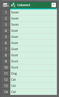
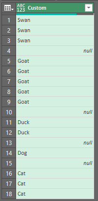
Is there a formula I can put into Column G (from G4 down) that will return what you can see in the picture? The formula is populating based on the criteria in Range C4:D8 and putting a blank cell between each animal type. A single formula would be great but I can work with intermediate helper cells/formula if necessary. I can work with a VBA solution if necessary but would like to see if there's a formula solution first (any VBA solution can't add rows).
Any help much appreciated.

 

[JvdV]

If I read correctly, you have data where you wish to add/delete rows on the go? If so, maybe for Excel2016 a PowerQuery solution could be a nice solution?

let
    Source = Excel.CurrentWorkbook(){[Name="Table1"]}[Content],
    #"Changed Type" = Table.TransformColumnTypes(Source,{{"Column1", type text}, {"Column2", Int64.Type}}),
    #"Added Custom" = Table.AddColumn(#"Changed Type", "Custom", each Table.Repeat(Table.FromRecords({[Col1=1]}), [Column2])),
    #"Expanded Custom" = Table.ExpandTableColumn(#"Added Custom", "Custom", {"Col1"}, {"Custom.Col1"}),
    #"Removed Columns" = Table.RemoveColumns(#"Expanded Custom",{"Column2", "Custom.Col1"})
in
    #"Removed Columns"

 

[awoohaw]

if text split and text join are in 2016, you can use this, it is not clean as it has some blank rows at the end.

mr excel questions 17.xlsm
	A	B	C	D	E	F	G	H
1
2
3
4			Swan	3			Swan
5			Goat	5			Swan
6			Duck	2			Swan
7			Dog	1
8			Cat	3			Goat
9							Goat
10							Goat
11							Goat
12							Goat
13
14							Duck
15							Duck
16
17							Dog
18
19							Cat
20							Cat
21							Cat
22
23
cjcass

Cell Formulas
Range	Formula
G4:G22	G4	=TEXTSPLIT(TEXTJOIN(",",,SUBSTITUTE(REPT(C4:C8,D4:D8)&",",RIGHT(C4:C8,1)&LEFT(C4:C8,1),RIGHT(C4:C8,1)&","&LEFT(C4:C8,1))),,",")
Dynamic array formulas.

 

[cjcass]

if text split and text join are in 2016, you can use this, it is not clean as it has some blank rows at the end.

mr excel questions 17.xlsm
	A	B	C	D	E	F	G	H
1
2
3
4			Swan	3			Swan
5			Goat	5			Swan
6			Duck	2			Swan
7			Dog	1
8			Cat	3			Goat
9							Goat
10							Goat
11							Goat
12							Goat
13
14							Duck
15							Duck
16
17							Dog
18
19							Cat
20							Cat
21							Cat
22
23
cjcass

Cell Formulas
Range	Formula
G4:G22	G4	=TEXTSPLIT(TEXTJOIN(",",,SUBSTITUTE(REPT(C4:C8,D4:D8)&",",RIGHT(C4:C8,1)&LEFT(C4:C8,1),RIGHT(C4:C8,1)&","&LEFT(C4:C8,1))),,",")
Dynamic array formulas.

Hi,
I entered your formula into G4 and it returns #NAME?

 

[awoohaw]

Hi,
I entered your formula into G4 and it returns #NAME?

okay, so some of the functions i use are not in 2016. I'll have to think of something else.

 

[JvdV]

I've just read/seen the intermediate whitespaces. Therefor the PQ solution would become a little longer:

let
    Source = Excel.CurrentWorkbook(){[Name="Table1"]}[Content],
    #"Changed Type" = Table.TransformColumnTypes(Source,{{"Column1", type text}, {"Column2", Int64.Type}}),
    #"Added Index" = Table.AddIndexColumn(#"Changed Type", "Index", 0, 1, Int64.Type),
    #"Added Custom" = Table.AddColumn(#"Added Index", "Custom", each Table.Repeat(Table.FromRecords({[Col1=1]}), [Column2])),
    #"Expanded Custom" = Table.ExpandTableColumn(#"Added Custom", "Custom", {"Col1"}, {"Custom.Col1"}),
    #"Appended Query" = Table.Combine({#"Expanded Custom", #"Added Index"}),
    #"Added Custom1" = Table.AddColumn(#"Appended Query", "Custom", each if [Custom.Col1] = 1 then[Column1] else null),
    #"Sorted Rows" = Table.Sort(#"Added Custom1",{{"Index", Order.Ascending}, {"Custom", Order.Descending}}),
    #"Removed Columns" = Table.RemoveColumns(#"Sorted Rows",{"Column1", "Column2", "Index", "Custom.Col1"}),
    #"Removed LastRow" = Table.RemoveLastN(#"Removed Columns", 1)
in
    #"Removed LastRow"

 

[cjcass]

If I read correctly, you have data where you wish to add/delete rows on the go? If so, maybe for Excel2016 a PowerQuery solution could be a nice solution?

let
    Source = Excel.CurrentWorkbook(){[Name="Table1"]}[Content],
    #"Changed Type" = Table.TransformColumnTypes(Source,{{"Column1", type text}, {"Column2", Int64.Type}}),
    #"Added Custom" = Table.AddColumn(#"Changed Type", "Custom", each Table.Repeat(Table.FromRecords({[Col1=1]}), [Column2])),
    #"Expanded Custom" = Table.ExpandTableColumn(#"Added Custom", "Custom", {"Col1"}, {"Custom.Col1"}),
    #"Removed Columns" = Table.RemoveColumns(#"Expanded Custom",{"Column2", "Custom.Col1"})
in
    #"Removed Columns"

Hi, I'm not wishing to add or delete any rows / columns in the solution and I'm also not familiar with or using PowerBI. I notice your solution hasn't left a gap between the animals. Maybe a standard VBA or formula solution?

 

[JvdV]

Hi, I'm not wishing to add or delete any rows / columns in the solution and I'm also not familiar with or using PowerBI. I notice your solution hasn't left a gap between the animals. Maybe a standard VBA or formula solution?

Yeah, just before your post I added an updated answer to include blank rows. You don't need to be very familiar with PowerQuery to be honest. If you click on either one of your animals you can load your little table into PQ using 'From Table/Range' option in the 'Get & Transform Data' group sitting on the 'Data' tab. Confirm you don't use headers (as per sample). In the screen that opens you'd just paste the above M-code in the 'Advanced Editor' in the 'View' tab. Only thing for you to check is that the name of the table you refer to will be "Table1".

 

[Fluff]

How about

Fluff.xlsm
	A	B	C	D	E	F	G
1
2
3
4			Swan	3	0		Swan
5			Goat	5	4		Swan
6			Duck	2	10		Swan
7			Dog	1	13
8			Cat	3	15		Goat
9							Goat
10							Goat
11							Goat
12							Goat
13
14							Duck
15							Duck
16
17							Dog
18
19							Cat
20
21
Summary

Cell Formulas
Range	Formula
E4:E10	E4	=IF(D4="","",SUM(D$3:D3)+ROWS(E$4:E4)-1)
G4:G21	G4	=IF(OR(ISNUMBER(MATCH(ROWS(G$4:G4),$E$4:$E$10,0)),ROWS(G$4:G4)>MAX($E$4:$E$10)+1),"",INDEX($C$4:$C$10,MATCH(ROWS(G$4:G4),$E$4:$E$10,1)))

 

[cjcass]

How about

Fluff.xlsm
	A	B	C	D	E	F	G
1
2
3
4			Swan	3	0		Swan
5			Goat	5	4		Swan
6			Duck	2	10		Swan
7			Dog	1	13
8			Cat	3	15		Goat
9							Goat
10							Goat
11							Goat
12							Goat
13
14							Duck
15							Duck
16
17							Dog
18
19							Cat
20
21
Summary

Cell Formulas
Range	Formula
E4:E10	E4	=IF(D4="","",SUM(D$3:D3)+ROWS(E$4:E4)-1)
G4:G21	G4	=IF(OR(ISNUMBER(MATCH(ROWS(G$4:G4),$E$4:$E$10,0)),ROWS(G$4:G4)>MAX($E$4:$E$10)+1),"",INDEX($C$4:$C$10,MATCH(ROWS(G$4:G4),$E$4:$E$10,1)))

Hi, that works well if I add a 'bogus' extra animal at the end then 'Cat' will populate 3 cells