Populate cells based on value in another tab

[Surferol]

Hi,
I have an index which contains data such as ID number, last survey, next survey due, days left till next survey.
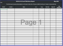
I want a separate monthly report tab to auto populate the ID numbers based on how long is left till the expiry date.
The monthly report tab is already set up to pull specific data from the index based on the IDs, I just need a way for the correct ID number to automatically populate the right column.
Thanks

 

[Toadstool]

Hi Surefrol,

Here's my INDEX tab with the data

Surferol.xlsx
	A	B	C	D
1	ID	Last Survey	Next Survey	Days Left to Next Survey
2	XS644	02-Feb-20	21-Apr-21	11
3	XS966	17-Mar-20	02-Mar-21	-39
4	XS492	30-Apr-20	15-Apr-21	5
5	XS615	13-Jun-20	28-Apr-21	18
6	XS738	27-Jul-20	12-Jul-21	93
7	XS861	09-Sep-20	25-Aug-21	137
8	XS984	23-Oct-20	28-Apr-21	18
9
INDEX

Cell Formulas
Range	Formula
D2:D8	D2	=C2-TODAY()

Here's my REPORT tabe with the results

Surferol.xlsx
	A	B
1	ID	Days Left to Next Survey
2	XS966	-39
3	XS492	5
4	XS644	11
5	XS615	18
6	XS984	18
7	XS738	93
8	XS861	137
9
REPORT

Cell Formulas
Range	Formula
A2:A9	A2	=IF(B2="","",INDEX(INDEX!$A$2:$A$9999,AGGREGATE(15,6,ROW(INDEX!$A$2:$A$9999)-ROW(INDEX!$A$1)/(INDEX!$D$2:$D$9999=B2),COUNTIF($B$1:$B2,B2))))
B2:B9	B2	=IFERROR(AGGREGATE(15,6,INDEX!$D$2:$D$9999,ROW()-ROW($A$1)),"")

 

[Surferol]

Thank you, that's awesome.
Does this also work if I only want the report to fill with info from anything that has less than 45 days left?

 

[Surferol]

Hi Toadstool,
This is an example of my data, you can see some of the entries had >45 days left, others are <45 days and some have no days remains (-31 and -499)
I would like the report to fill in just the ID number (the rest of that page will pull the remaining info already), but only for the entries that have less than 45 days remaining.

 

[Fluff]

How about

+Fluff 1.xlsm
	A	B	C	D
1	ID	Last Survey	Next Survey	Days Left to Next Survey
2	XS644	02/02/2020	21/04/2021	10
3	XS966	17/03/2020	02/03/2021	-40
4	XS492	30/04/2020	15/04/2021	4
5	XS615	13/06/2020	28/04/2021	17
6	XS738	27/07/2020	12/07/2021	92
7	XS861	09/09/2020	25/08/2021	136
8	XS984	23/10/2020	28/04/2021	17
9
10
Main

Cell Formulas
Range	Formula
D2:D8	D2	=C2-TODAY()

+Fluff 1.xlsm
	A
1	ID
2	XS644
3	XS966
4	XS492
5	XS615
6	XS984
7
Summary

Cell Formulas
Range	Formula
A2:A6	A2	=FILTER(Main!A2:A100,(Main!D2:D100<45)*(Main!A2:A100<>""))
Dynamic array formulas.

 

[Surferol]

Fluff,
That worked perfectly, Thank you.

 

[Fluff]

You're welcome & thanks for the feedback.