Pragmatically putting VLOOKUP in Formula does not work

[DragonSoft]

(Note: I'm not allowed to install XL2BB on a company computer so pics will have to do)

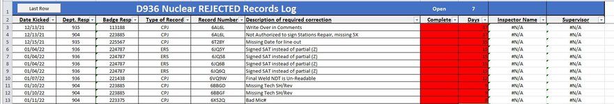
Using the below code to put VLOOKUP in two columns (I & J) has stopped working. The formula IS put in each cell but the results is always #N/A even after verifying the look up value is in the table.
I am ONLY interested it the rows that have 936 in Column B (Dept.Resp)

Private Sub Auto_Open()

    'Call Show_Screens(False)
    Last_Row = 3 'skip the header rows
    Set This_WorkSheet = Workbooks(ActiveWorkbook.Name).Worksheets("Data")      ' Data Sheet
    Last_Row = This_WorkSheet.Cells(This_WorkSheet.Rows.Count, "A").End(xlUp).Offset(0).Row

    Sheets("Data").Select                                   ' Select and Display the Data Sheet
    Range("A2").Select                                      ' Select the Active Cell
    MyRange = "A3:J" & Last_Row                             ' Set our Sort Range

    Range(MyRange).Select
    ActiveWorkbook.Worksheets("Data").Sort.SortFields.Clear
    ActiveWorkbook.Worksheets("Data").Sort.SortFields.Add(Range("G3:G" & Last_Row), _
        xlSortOnCellColor, xlAscending, , xlSortNormal).SortOnValue.Color = RGB(255, 0 _
        , 0)
    ActiveWorkbook.Worksheets("Data").Sort.SortFields.Add Key:=Range("G3:G" & Last_Row), _
        SortOn:=xlSortOnValues, Order:=xlAscending, DataOption:=xlSortNormal
    With ActiveWorkbook.Worksheets("Data").Sort
        .SetRange Range("A2:J" & Last_Row)
        .Header = xlYes
        .MatchCase = False
        .Orientation = xlTopToBottom
        .SortMethod = xlPinYin
        .Apply
    End With
    For N = 3 To Last_Row
        Worksheets("Data").Range("I" & N).Formula = "=VLOOKUP(C" & N & ", Inspectors!A3:F115,2,)"
        '=VLOOKUP(A2,Inspectors!A3:F115,2,)
        Worksheets("Data").Range("J" & N).Formula = "=VLOOKUP(C" & N & ", Inspectors!A3:F115,6,)"
    Next N
    Sheets("Data").Select                                   ' Select and Display the NDT Sheet
    Range("A3").Select                                      ' Select the Active Cell
End Sub

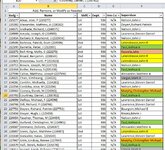
Data Tab and Inspector Tab pictures attached

 

[DragonSoft]

Adding a pic showing the formula that gets put in the cell

 

[Peter_SSs]

It looks like in one sheet the column might be numerical and in the other the column might be "numbers stored as text"

What happens if you make changes like this?

Worksheets("Data").Range("I" & N).Formula = "=VLOOKUP(C" & N & ", Inspectors!A3:F115,2,)"
Worksheets("Data").Range("I" & N).Formula = "=VLOOKUP(C" & N & "+0, Inspectors!A3:F115,2,)"

 

[DragonSoft]

It looks like in one sheet the column might be numerical and in the other the column might be "numbers stored as text"

What happens if you make changes like this?

Worksheets("Data").Range("I" & N).Formula = "=VLOOKUP(C" & N & ", Inspectors!A3:F115,2,)"
Worksheets("Data").Range("I" & N).Formula = "=VLOOKUP(C" & N & "+0, Inspectors!A3:F115,2,)"

Perfect! That fixed it! Thanks or your help. Now I just need to put it in an IF statement (boss does not like seeing the #N/A's.

 

[Peter_SSs]

I would use the IFNA function rather than IF.

eg

Worksheets("Data").Range("I" & N).Formula = "=IFNA(VLOOKUP(C" & N & "+0, Inspectors!A3:F115,2,),"""")"

 

[DragonSoft]

I would use the IFNA function rather than IF.

eg

Worksheets("Data").Range("I" & N).Formula = "=IFNA(VLOOKUP(C" & N & "+0, Inspectors!A3:F115,2,),"""")"

Thanks that works great. I had just nested the vlookup in a IF("B" & N = 936) ... But I'm always interested in learning new functions.