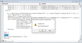
Private Sub Worksheet_Change(ByVal Target As Range)
Dim i As Long, j As Long, Lr1 As Long, Lr2 As Long, Cr1 As Long, Cr1R As String, Cr2 As Long, Cr2R As String
Dim Lr3 As Long, Lr4 As Long, M1 As Long, M2 As Long, Cr3 As Variant
On Error Resume Next
Lr1 = Range("I" & Rows.Count).End(xlUp).Row + Target.Rows.Count - 1
Lr2 = Range("N" & Rows.Count).End(xlUp).Row + Target.Rows.Count - 1
If Intersect(Target, Union(Range("I3:I" & Lr1 - 1), Range("N3:N" & Lr2 - 1))) Is Nothing Then Exit Sub
Lr3 = Sheets("Work").Range("A" & Rows.Count).End(xlUp).Row
Lr4 = Sheets("Paper").Range("A" & Rows.Count).End(xlUp).Row
If Target.Count > 1 Then
Application.EnableEvents = False
If Not Intersect(Target, Range("I3:I" & Lr1 - 1)) Is Nothing Then
M1 = Application.WorksheetFunction.Match(Range("I" & Target.Row - 1), Sheets("Work").Range("A1:A" & Lr3), 0)
If M1 = 0 Then
M1 = 1
GoTo Resum2
End If
For i = M1 + 2 To Lr3
If Sheets("work").Range("A" & i).Interior.Color = 4697456 Then
M1 = i
GoTo Resum2
End If
Next i
Resum2:
M2 = Application.WorksheetFunction.Match(Range("I" & Target.Row), Sheets("Work").Range("A1:A" & Lr3), 0) - 1
Sheets("Work").Rows(M1 & ":" & M2).Delete
For i = Target.Row To Lr1 - Target.Rows.Count
  If i = 3 Then
     Range("J" & i).FormulaR1C1 = "=IFERROR(INDEX(Work!C[-8],MATCH(R[1]C9,Work!C[-9],0)-2,0),"""")"
     Range("K" & i).FormulaR1C1 = "=IFERROR(SUM(INDEX(Work!C[-7],MATCH(RC9,Work!C[-10],0)+1,0):INDEX(Work!C[-6],MATCH(R[1]C9,Work!C[-10],0)-2,0)),"""")"
     Range("L" & i).FormulaR1C1 = "=IFERROR(SUM(INDEX(Work!C[-6],MATCH(RC9,Work!C[-11],0)+1,0):INDEX(Work!C[-5],MATCH(R[1]C9,Work!C[-11],0)-2,0)),"""")"
  ElseIf i > 3 Then
     Range("J" & i - 1 & ":J" & i).FormulaR1C1 = "=IFERROR(INDEX(Work!C[-8],MATCH(R[1]C9,Work!C[-9],0)-2,0),"""")"
     Range("K" & i - 1 & ":K" & i).FormulaR1C1 = "=IFERROR(SUM(INDEX(Work!C[-7],MATCH(RC9,Work!C[-10],0)+1,0):INDEX(Work!C[-6],MATCH(R[1]C9,Work!C[-10],0)-2,0)),"""")"
     Range("L" & i - 1 & ":L" & i).FormulaR1C1 = "=IFERROR(SUM(INDEX(Work!C[-6],MATCH(RC9,Work!C[-11],0)+1,0):INDEX(Work!C[-5],MATCH(R[1]C9,Work!C[-11],0)-2,0)),"""")"
  End If

    Cr1 = Application.WorksheetFunction.Match(Range("I" & i), Sheets("Work").Range("A1:A" & Lr3), 0)
     Cr1R = Range("A" & Cr1).Address
     Range("I" & i).Hyperlinks.Delete
     Sheets("Dashboard").Hyperlinks.Add Anchor:=Range("I" & i), Address:="", SubAddress:="'" & Sheets("Work").Name & "'!" & Cr1R, TextToDisplay:=Range("I" & i).Value
     With Sheets("Dashboard").Range("I" & i)
                .Font.Underline = xlUnderlineStyleNone
                .Font.ColorIndex = xlColorIndexAutomatic
                .Font.Name = "Arial"
                .Font.Size = 14
                .HorizontalAlignment = xlCenter
                .VerticalAlignment = xlCenter
     End With

Next i
End If

If Not Intersect(Target, Range("N3:N" & Lr2 - 1)) Is Nothing Then
M1 = Application.WorksheetFunction.Match(Range("N" & Target.Row - 1), Sheets("Paper").Range("A1:A" & Lr4), 0)
If M1 = 0 Then
M1 = 1
GoTo Resum3
End If
For i = M1 + 2 To Lr3
If Sheets("Paper").Range("A" & i).Interior.Color = 12874308 Then
M1 = i
GoTo Resum3
End If
Next i
Resum3:
M2 = Application.WorksheetFunction.Match(Range("N" & Target.Row), Sheets("Paper").Range("A1:A" & Lr4), 0) - 1
Sheets("Paper").Rows(M1 & ":" & M2).Delete
For i = Target.Row To Lr2 - Target.Rows.Count
  If i = 3 Then
     Range("O" & i).FormulaR1C1 = "=IFERROR(INDEX(Paper!C[-13],MATCH(R[1]C14,Paper!C[-14],0)-2,0),"""")"
     Range("P" & i).FormulaR1C1 = "=IFERROR(SUM(INDEX(Paper!C[-12],MATCH(RC14,Paper!C[-15],0)+1,0):INDEX(Paper!C[-11],MATCH(R[1]C14,Paper!C[-15],0)-2,0)),"""")"
     Range("Q" & i).FormulaR1C1 = "=IFERROR(SUM(INDEX(Paper!C[-11],MATCH(RC14,Paper!C[-16],0)+1,0):INDEX(Paper!C[-10],MATCH(R[1]C14,Paper!C[-16],0)-2,0)),"""")"
  ElseIf i > 3 Then
     Range("O" & i - 1 & ":O" & i).FormulaR1C1 = "=IFERROR(INDEX(Paper!C[-13],MATCH(R[1]C14,Paper!C[-14],0)-2,0),"""")"
     Range("P" & i - 1 & ":P" & i).FormulaR1C1 = "=IFERROR(SUM(INDEX(Paper!C[-12],MATCH(RC14,Paper!C[-15],0)+1,0):INDEX(Paper!C[-11],MATCH(R[1]C14,Paper!C[-15],0)-2,0)),"""")"
     Range("Q" & i - 1 & ":Q" & i).FormulaR1C1 = "=IFERROR(SUM(INDEX(Paper!C[-11],MATCH(RC14,Paper!C[-16],0)+1,0):INDEX(Paper!C[-10],MATCH(R[1]C14,Paper!C[-16],0)-2,0)),"""")"
  End If

    Cr1 = Application.WorksheetFunction.Match(Range("N" & i), Sheets("Paper").Range("A1:A" & Lr4), 0)
     Cr1R = Range("A" & Cr1).Address
     Range("N" & i).Hyperlinks.Delete
     Sheets("Dashboard").Hyperlinks.Add Anchor:=Range("N" & i), Address:="", SubAddress:="'" & Sheets("Paper").Name & "'!" & Cr1R, TextToDisplay:=Range("N" & i).Value
     With Sheets("Dashboard").Range("N" & i)
                .Font.Underline = xlUnderlineStyleNone
                .Font.ColorIndex = xlColorIndexAutomatic
                .Font.Name = "Arial"
                .Font.Size = 14
                .HorizontalAlignment = xlCenter
                .VerticalAlignment = xlCenter
     End With

Next i
End If
End If
Application.EnableEvents = True
End Sub
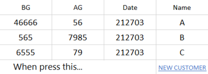
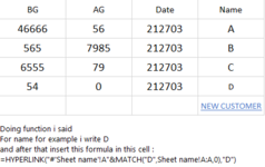
") Thank you for give your time...
Thank you for give your time...


