PROBLEM SUMIF ARRAY IN RESULT

roykana

Active Member
Joined
Mar 8, 2018
Messages
311
Office Version
  1. 2010
Platform
  1. Windows
Dear All Master,
It should be in column B in the "recon" sheet which I mark yellow but I use the vba code below but the result is in column G in the sheet "recon" which I mark red. There may be something wrong in the code I edited below and I just added a little or modified it a little without changing the code structure below.

thanks
roykana

VBA Code:
Option Explicit

Sub SumIfs()
  Dim dic As Object
  Dim shs As Variant
  Dim a As Variant, b As Variant, c As Variant, d As Variant
  Dim i As Long, j As Long, k As Long, lr As Long, lt As Long, m As Long, n As Long
  
  Set dic = CreateObject("Scripting.Dictionary")
  shs = Array("TEST", "A")
  
  For i = 0 To UBound(shs) Step 2
    'Find the last row with data from each sheet.
    lr = Sheets(shs(i)).Range(shs(i + 1) & Rows.Count).End(3).Row
    'Calculate the possible total of rows, that is, the sum of the rows of all the sheets
    lt = lt + lr
    'Fill a matrix for each sheet
    If i = 0 Then a = Sheets(shs(i)).Range("A2:G" & lr).Value

  Next
  
  'To fill everything with 0
  ReDim d(1 To lt + 1, 1 To 7)
  For i = 1 To UBound(d, 1)
    For j = 2 To UBound(d, 2)
      d(i, j) = 0
    Next
  Next
  
  'OPS
  For i = 1 To UBound(a, 1)
    If Not dic.exists(a(i, 1)) Then
      'If it is not in the dictionary, the row of the output matrix is ??increased by one
      n = n + 1
      'The dictionary is filled with the row number
      dic(a(i, 1)) = n
      'The array is filled, the value is put in the row number, column 1
      d(n, 1) = a(i, 1)
    End If
    'Gets the row number in j
    j = dic(a(i, 1))
    For k = 7 To 7
      'The values are added within the matrix, in row j, from column 7 to column 7
      d(j, k) = d(j, k) + a(i, k)
    Next
  Next
  
  
  'Calculate totals
  k = n + 1
  For i = 1 To n
    For j = 2 To UBound(d, 2)
      d(k, j) = d(k, j) + d(i, j)
    Next
  Next

  Sheets("RECON").Range("A2").Resize(n + 1, UBound(d, 2)).Value = d
End Sub

Source
problem sumif.xlsm
ABCDEFG
1ITEM NOITEM 1ITC 1ITEM 2ITC 2QM18QCJR
21000TEST R 10000-1000TEST RR 10000-1000-055
31001TEST R 10010-1001TEST RR 10010-1001-01010
TEST


DESIRED RESULT
problem sumif.xlsm
ABCDEFG
1ITEM NOQCJR
21000000005
310010000010
40000015
RECON
 

Excel Facts

Ambidextrous Undo
Undo last command with Ctrl+Z or Alt+Backspace. If you use the Undo icon in the QAT, open the drop-down arrow to undo up to 100 steps.
I think you're trying to do a simple SUMIF, like this perhaps? If I'm correct, your code can be made much simpler.

Input
ABCDEFG
1ITEM NOITEM 1ITC 1ITEM 2ITC 2QM18QCJR
210005
3100110
410003
510007
6100111
7100213
TEST

Output?
AB
1ITEM NOQCJR
2100015
3100121
4100213
RECON
 
Upvote 0
I think you're trying to do a simple SUMIF, like this perhaps? If I'm correct, your code can be made much simpler.

Input
ABCDEFG
1ITEM NOITEM 1ITC 1ITEM 2ITC 2QM18QCJR
210005
3100110
410003
510007
6100111
7100213
TEST

Output?
AB
1ITEM NOQCJR
2100015
3100121
4100213
RECON
@StephenCrump
That's right. Actually previously the code was used for multi sheet for sumif and sumifs but I have eliminated other codes but certainly in the future for multi sheet and multi criteris. If you can modify it a little it's better. Maybe if you have better recommendations but still use arrays and dictionaries so that it is faster
 
Upvote 0
Using my layout in Post #2, try:

VBA Code:
Sub Test()

    Dim vIn As Variant
    Dim dic As Object
    Dim i As Long
    Const COL = 7   'column G
        
    Set dic = CreateObject("Scripting.Dictionary")
    dic.CompareMode = vbTextCompare

    With Worksheets("TEST")
        vIn = .Range("A2:A" & .Range("A" & Rows.Count).End(xlUp).Row).Resize(, COL).Value2
    End With

    For i = 1 To UBound(vIn)
        dic(vIn(i, 1)) = dic(vIn(i, 1)) + vIn(i, COL)
    Next i
    
    With Worksheets("RECON").Range("A2").Resize(dic.Count)
        .Value = Application.Transpose(dic.Keys)
        .Offset(, 1).Value = Application.Transpose(dic.Items)
    End With
    
End Sub
 
Upvote 0
Using my layout in Post #2, try:

VBA Code:
Sub Test()

    Dim vIn As Variant
    Dim dic As Object
    Dim i As Long
    Const COL = 7   'column G
      
    Set dic = CreateObject("Scripting.Dictionary")
    dic.CompareMode = vbTextCompare

    With Worksheets("TEST")
        vIn = .Range("A2:A" & .Range("A" & Rows.Count).End(xlUp).Row).Resize(, COL).Value2
    End With

    For i = 1 To UBound(vIn)
        dic(vIn(i, 1)) = dic(vIn(i, 1)) + vIn(i, COL)
    Next i
  
    With Worksheets("RECON").Range("A2").Resize(dic.Count)
        .Value = Application.Transpose(dic.Keys)
        .Offset(, 1).Value = Application.Transpose(dic.Items)
    End With
  
End Sub
@StephenCrump
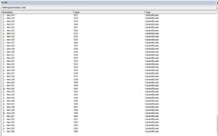
I've tried the code successfully but if I try for 100000 records there is an error (run time error 13) in the code below
is there a limit and I also attach screenshots.
VBA Code:
        .Value = Application.Transpose(dic.Keys)
 

Attachments

  • Capture04-02-2022.JPG
    Capture04-02-2022.JPG
    89.6 KB · Views: 9
Upvote 0
Yes, too many to TRANSPOSE.

Try:

VBA Code:
Sub Test()

    Dim vIn As Variant, vOut As Variant, key As Variant
    Dim dic As Object
    Dim i As Long
    Const COL = 7   'column G
        
    Set dic = CreateObject("Scripting.Dictionary")
    dic.CompareMode = vbTextCompare

    With Worksheets("TEST")
        vIn = .Range("A2:A" & .Range("A" & Rows.Count).End(xlUp).Row).Resize(, COL).Value2
    End With

    For i = 1 To UBound(vIn)
        dic(vIn(i, 1)) = dic(vIn(i, 1)) + vIn(i, COL)
    Next i
    
    ReDim vOut(1 To dic.Count, 1 To 2)
    i = 1
    For Each key In dic.keys
        vOut(i, 1) = key
        vOut(i, 2) = dic(key)
        i = i + 1
    Next key
    Worksheets("RECON").Range("A2").Resize(dic.Count, 2).Value = vOut
    
End Sub
 
Upvote 0
Yes, too many to TRANSPOSE.

Try:

VBA Code:
Sub Test()

    Dim vIn As Variant, vOut As Variant, key As Variant
    Dim dic As Object
    Dim i As Long
    Const COL = 7   'column G
       
    Set dic = CreateObject("Scripting.Dictionary")
    dic.CompareMode = vbTextCompare

    With Worksheets("TEST")
        vIn = .Range("A2:A" & .Range("A" & Rows.Count).End(xlUp).Row).Resize(, COL).Value2
    End With

    For i = 1 To UBound(vIn)
        dic(vIn(i, 1)) = dic(vIn(i, 1)) + vIn(i, COL)
    Next i
   
    ReDim vOut(1 To dic.Count, 1 To 2)
    i = 1
    For Each key In dic.keys
        vOut(i, 1) = key
        vOut(i, 2) = dic(key)
        i = i + 1
    Next key
    Worksheets("RECON").Range("A2").Resize(dic.Count, 2).Value = vOut
   
End Sub
@StephenCrump
Thanks for the reply from you, sorry if I'm late reply, it went perfectly.
from your code I want to do multi source with sumif & sumifs, for the yellow color that is in the source it is the value (sum_range) and for the orange color that is in the source it is a criterion. For the sheet "RECON" that I mark the blue color it is the desired result and also I use the formula so that it is easy to understand.

thanks
roykana

Source1
problem sumif.xlsm
ABCDEFG
1ITEM NOITEM 1ITC 1ITEM 2ITC 2QM18QCJR
21000TEST R 10000-1000TEST RR 10000-1000-055
31001TEST R 10010-1001TEST RR 10010-1001-01010
41515
TEST
Cell Formulas
RangeFormula
F4F4=SUBTOTAL(109,[QM18])
G4G4=SUBTOTAL(109,[QCJR])

Source2
problem sumif.xlsm
ABCDEFGHIJKLMNOPQ
1PNMITMITCQTYUNICIUNODDPRNCURQABGLBDPTDATESACDEPTTRANSITEM NO
2U-1000TEST R 100010001005-02-221M01PURCHASE1000
3U-1001TEST R 100110011505-02-222N01PURCHASE1001
4U-1002TEST R 100010001305-02-223O01PURCHASE1000
5U-1003TEST R 100110011205-02-224P01PURCHASE1001
6U-1004TEST R 100010001105-02-225M01SALES1000
7U-1005TEST R 100110011305-02-226N01SALES1001
8U-1006TEST R 100010001505-02-227O01SALES1000
9U-1007TEST R 100110011805-02-228P01SALES1001
10107
MUTATION
Cell Formulas
RangeFormula
D10D10=SUBTOTAL(109,[QTY])

Source3
problem sumif.xlsm
ABCDEFG
1ITCITMQFSKINVREMARKITEM NOGROUP
21000TEST R 1000101000BOJ
31001TEST R 1001151001M18
41003TEST R 1003251003BOJ
51000TEST R 1000111000CJR
61001TEST R 1001121001CJR
773
MUTATION1
Cell Formulas
RangeFormula
C7C7=SUBTOTAL(109,[QFSK])


Desired result
problem sumif.xlsm
ABCDEFGHIJKLM
1ITEM NOQJRPURCHASESALESBOJCJRM18
2M01N01O01P01M01N01O01P01
31000510013011015010110
410011001501201301801215
5651015131211131518102315
RECON
Cell Formulas
RangeFormula
C3:F4C3=SUMIFS(MUTATION[QTY],MUTATION[ITEM NO],$A3,MUTATION[TRANS],RECON!$C$1,MUTATION[DEPT],RECON!C$2)
G3:J4G3=SUMIFS(MUTATION[QTY],MUTATION[ITEM NO],$A3,MUTATION[TRANS],RECON!$G$1,MUTATION[DEPT],RECON!G$2)
K3:M4K3=SUMIFS(MUTATION1[QFSK],MUTATION1[ITEM NO],RECON!$A3,MUTATION1[GROUP],RECON!K$1)
C5:M5C5=SUM(C3:C4)
 
Upvote 0
That's great, I'm glad it worked for you.

Sorry, I don't have the time for your follow up question - it will require quite a bit more work to implement in VBA. Normally I'd suggest starting a new thread, but I see that you have already started several similar threads recently.

Bottom line: if your workbook is so unwieldy that you think you should replace all your (dynamic) Excel formulae with (static) VBA results, you probably should be using alternatives such as Power Pivot.
@StephenCrump
Thank you for your reply. if using the code below then I can do multi source as I want, so I want the code structure below does not need to be changed just modify a little so that the result can be the same as the output I want
VBA Code:
Option Explicit

Sub SumIfs()
  Dim dic As Object
  Dim shs As Variant
  Dim a As Variant, b As Variant, c As Variant, d As Variant
  Dim i As Long, j As Long, k As Long, lr As Long, lt As Long, m As Long, n As Long
  
  Set dic = CreateObject("Scripting.Dictionary")
  shs = Array("TEST", "A")
  
  For i = 0 To UBound(shs) Step 2
    'Find the last row with data from each sheet.
    lr = Sheets(shs(i)).Range(shs(i + 1) & Rows.Count).End(3).Row
    'Calculate the possible total of rows, that is, the sum of the rows of all the sheets
    lt = lt + lr
    'Fill a matrix for each sheet
    If i = 0 Then a = Sheets(shs(i)).Range("A2:G" & lr).Value

  Next
  
  'To fill everything with 0
  ReDim d(1 To lt + 1, 1 To 7)
  For i = 1 To UBound(d, 1)
    For j = 2 To UBound(d, 2)
      d(i, j) = 0
    Next
  Next
  
  'TEST
  For i = 1 To UBound(a, 1)
    If Not dic.exists(a(i, 1)) Then
      'If it is not in the dictionary, the row of the output matrix is ??increased by one
      n = n + 1
      'The dictionary is filled with the row number
      dic(a(i, 1)) = n
      'The array is filled, the value is put in the row number, column 1
      d(n, 1) = a(i, 1)
    End If
    'Gets the row number in j
    j = dic(a(i, 1))
    For k = 7 To 7
      'The values are added within the matrix, in row j, from column 7 to column 7
      d(j, k) = d(j, k) + a(i, k)
    Next
  Next
  
  
  'Calculate totals
  k = n + 1
  For i = 1 To n
    For j = 2 To UBound(d, 2)
      d(k, j) = d(k, j) + d(i, j)
    Next
  Next

  Sheets("RECON").Range("A2").Resize(n + 1, UBound(d, 2)).Value = d
End Sub
 
Upvote 0

Forum statistics

Threads
1,214,642
Messages
6,120,701
Members
448,980
Latest member
CarlosWin

We've detected that you are using an adblocker.

We have a great community of people providing Excel help here, but the hosting costs are enormous. You can help keep this site running by allowing ads on MrExcel.com.
Allow Ads at MrExcel

Which adblocker are you using?

Disable AdBlock

Follow these easy steps to disable AdBlock

1)Click on the icon in the browser’s toolbar.
2)Click on the icon in the browser’s toolbar.
2)Click on the "Pause on this site" option.
Go back

Disable AdBlock Plus

Follow these easy steps to disable AdBlock Plus

1)Click on the icon in the browser’s toolbar.
2)Click on the toggle to disable it for "mrexcel.com".
Go back

Disable uBlock Origin

Follow these easy steps to disable uBlock Origin

1)Click on the icon in the browser’s toolbar.
2)Click on the "Power" button.
3)Click on the "Refresh" button.
Go back

Disable uBlock

Follow these easy steps to disable uBlock

1)Click on the icon in the browser’s toolbar.
2)Click on the "Power" button.
3)Click on the "Refresh" button.
Go back
Back
Top