Problem with sales, multiple values, postcodes, etc.

[Tashbbb]

Hi guys,


I came across this problem today and I'm not sure how to solve it..I'm sure this is easy for you but I'm a beginner so this is really stressing me out ((

I have two tabs which include:

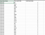
1: Sales dates, postcodes and number of sales

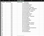
2: postcodes, store number, store names

Each postcodes is associated with a certain store number and store numbers is associated with a store name.
Now....

1)How do I get total number of sales per store (name)?

2)How do I calculate which two months had the highest volume of sales taking only into consideration stores that had sales from September onwards? (and excluding stores which are not associate with a postcode)?

3) How do I figure out which store had the fastest growth?

Number 1 and 2 are giving me more headaches...I tried to look online but I cannot find a solution

I really appreciate your help !!!!

 

[CA_Punit]

1st Question: 1 Create a store Id Helper Column in (Marked in Yellow) and use Sumif function as stated in column F and it will give you total Number of Sales (Assuming Column P is Count of Sales and Not the sales volume)

2nd Question use the Formula used in R2 and i have considered sales volume beginning from 01/09/2019 and the dates correspondence to only one Financial or calender year.

 

[CA_Punit]

In case of Formula in R2 please use Ctrl+Shift+Enter and not just Enter and drag it down.

 

[Tashbbb]

In case of Formula in R2 please use Ctrl+Shift+Enter and not just Enter and drag it down.

I tried to copy and paste and type cmd+shift+ enter, cmd + return, cmd + shift + return but none of these work...
Any suggestion? I have a mac and Excel 16.39

2.) Note Excluding new stores launched 2019, i.e., taking only stores that were active since September 2018, I need to know which two months had the highest volume of sales

 

[CA_Punit]

You dont have to type.
As you press enter once you are complete with the formula, here you have to press not just enter but Ctrl+Shift+Enter

 

[CA_Punit]

2.) Note Excluding new stores launched 2019, i.e., taking only stores that were active since September 2018, I need to know which two months had the highest volume of sales

You can just type the formula in Column S as =MONTH(N2)&" "&YEAR(N2) it will give 9 2019 and now you are ready for Pivot
just as shown in screenshot

 

[Fluff]

One way
add two helpers on the Data sheet

problem_forum.xlsx
	A	B	C	D	E
1	Data Month Sale	Post code Prefix	Confirmed Sales	date	store
2	2019-05	N7	1	01/05/2019	255
3	2019-05	SE12	1	01/05/2019	TBC
4	2019-05	BR6	1	01/05/2019	TBC
5	2019-05	SW16	1	01/05/2019	144
6	2019-05	BA1	1	01/05/2019	264
7	2019-05	SN1	1	01/05/2019	264
8	2019-05	M16	1	01/05/2019	186
9	2019-05	E1	1	01/05/2019	TBC
10	2019-05	NW6	1	01/05/2019	141
11	2019-05	W9	1	01/05/2019	141
12	2019-05	SW6	1	01/05/2019	144
13	2019-05	W12	1	01/05/2019	141
14	2019-05	KT14	2	01/05/2019	144
Data set

Cell Formulas
Range	Formula
D2:D14	D2	=DATE(LEFT(A2,4),RIGHT(A2,2),1)
E2:E14	E2	=VLOOKUP(B2,Lookup!$A$2:$B$1696,2,0)

And then on the Location sheet

problem_forum.xlsx
	D	E	F	G	H	I	J	K	L	M	N	O	P	Q	R	S	T
1	Store number	Store name		Sept	Oct	Nov	Dec	Jan	Feb	Mar	Apr	May	Jun	Jul	Aug
2	113	Store Belfast
3	125	Store Southampton
4	140	Store Warrington	ok	2	3	6	20	30	22	21	33	32	0	0	0	Apr	May
5	141	Store London - Wembley	ok	706	763	719	604	721	619	738	699	671	0	0	0	Oct	Mar
6	142	Store Birmingham - Wednesbury
7	143	Store Newcastle - Gateshead
8	144	Store London - Croydon	ok	527	584	538	530	525	490	570	562	551	0	0	0	Oct	Mar
9	150	Store Coventry
10	185	Store Milton Keynes	ok	5	2	8	6	5	4	3	5	4	0	0	0	Nov	Dec
11	186	Store Manchester	ok	80	82	85	67	71	75	160	164	145	0	0	0	Apr	Mar
12	255	Store London - Tottenham	ok	316	412	426	381	388	327	442	440	397	0	0	0	Mar	Apr
13	261	Store Leeds
14	262	Store Lakeside	ok	107	150	167	160	165	164	175	190	173	0	0	0	Apr	Mar
15	263	Store Nottingham
16	264	Store Bristol	ok	136	142	123	105	127	108	156	129	148	0	0	0	Mar	May
17	265	Store Edinburgh - Straiton
18	266	Store Glasgow - Braehead
19	267	Store Cardiff
20	461	Store Reading	ok	6	3	3	122	182	169	199	187	184	0	0	0	Mar	Apr
21	472	Store eCommerce Great Britain
22	519	Store Sheffield
23	548	Store Exeter
24	567	Store Greenwich
Lookup

Cell Formulas
Range	Formula
F2:F24	F2	=IF(COUNTIFS('Data set'!$E$2:$E$22500,D2,'Data set'!$D$2:$D$22500,"<=01/09/2018"),"ok","")
G2:R24	G2	=IF($F2="ok",SUMIFS('Data set'!$C$2:$C$22500,'Data set'!$E$2:$E$22500,$D2,'Data set'!$D$2:$D$22500,">="&DATE(2018,COLUMN(I1),1),'Data set'!$D$2:$D$22500,"<"&DATE(2018,COLUMN(J1),1)),"")
S2:T24	S2	=IF($F2="ok",INDEX($G$1:$R$1,MATCH(LARGE($G2:$R2,COLUMN(A1)),$G2:$R2,0)),"")

Using the helper columns, avoids the use of array formula which won't take kindly to working with over 22,000 rows.

 

[Tashbbb]

Thank you guys, I think I'm getting there....see below

How can I get the sales per month per each store (including all dates/months) ? I need to calculate the growth of each store so I guess it would make things easier.

So it's like
Sales Septmber 2018. Sales October 2018 Sales November. ..... 2019.... Growth
store xxx 10 20 30 ....... ........... 34. %


Look up:

problem_forum in progress.xlsx
	A	B	C	D	E	F	G	H	I	J	K	L	M	N	O	P	Q	R	S	T	U	V	W
1	Postcodes	Store number		Store number	Store name	Total volume sales Sep18-May 2019	Growth Sep 18-May 2019	Two month with highest volume of sales(stores launched from 2018 only)						Data Month Sale	Post code Prefix	Confirmed Sales	Store ID	Required sales/Sales per store	Date	Equal or less 2018?	Month	Year
2	BT1	113		113	Store Belfast	0								2019-05	N7	1	255	0	5/1/19		5	2019
3	BT10	113		125	Store Southampton	3								2019-05	SE12	1	TBC	0	5/1/19
4	BT11	113		140	Store Warrington	169								2019-05	BR6	1	TBC	0	5/1/19	ok
5	BT12	113		141	Store London - Wembley	6240								2019-05	SW16	1	144	0	5/1/19	ok
6	BT13	113		142	Store Birmingham - Wednesbury	464								2019-05	BA1	1	264	0	5/1/19
7	BT14	113		143	Store Newcastle - Gateshead	0								2019-05	SN1	1	264	0	5/1/19
8	BT15	113		144	Store London - Croydon	4877								2019-05	M16	1	186	0	5/1/19	ok
9	BT16	113		150	Store Coventry	270								2019-05	E1	1	TBC	0	5/1/19
10	BT17	113		185	Store Milton Keynes	42								2019-05	NW6	1	141	0	5/1/19	ok
11	BT18	113		186	Store Manchester	929								2019-05	W9	1	141	0	5/1/19	ok
12	BT19	113		255	Store London - Tottenham	3529								2019-05	SW6	1	144	0	5/1/19	ok
13	BT2	113		261	Store Leeds	0								2019-05	W12	1	141	0	5/1/19
14	BT20	113		262	Store Lakeside	1451								2019-05	KT14	2	144	0	5/1/19	ok
15	BT21	113		263	Store Nottingham	4								2019-05	KT12	3	144	0	5/1/19
16	BT22	113		264	Store Bristol	1174								2019-05	N9	1	255	0	5/1/19	ok
17	BT23	113		265	Store Edinburgh - Straiton	108								2019-05	E14	2	TBC	0	5/1/19
18	BT24	113		266	Store Glasgow - Braehead	79								2019-05	CR3	1	144	0	5/1/19
19	BT25	113		267	Store Cardiff	530								2019-05	SG12	1	255	0	5/1/19
20	BT26	113		461	Store Reading	1055								2019-05	B36	1	142	0	5/1/19	ok
21	BT27	113		472	Store eCommerce Great Britain	0								2019-05	N13	1	255	0	5/1/19
22	BT28	113		519	Store Sheffield	0								2019-05	N19	1	255	0	5/1/19
23	BT29	113		548	Store Exeter	0								2019-05	OX2	1	461	0	5/1/19
24	BT3	113		567	Store Greenwich	0								2019-05	SE1	1	144	0	5/1/19
25	BT30	113												2019-05	W8	2	141	0	5/1/19
26	BT36	113												2019-05	RM4	1	262	0	5/1/19
27	BT37	113												2019-05	WD25	1	141	0	5/1/19
28	BT38	113												2019-05	SE3	1	TBC	0	5/1/19
29	BT39	113												2019-05	TN15	1	TBC	0	5/1/19
Lookup

Cell Formulas
Range	Formula
Q2:Q29	Q2	=VLOOKUP(O2,A:B,2,FALSE)
R2	R2	=IFERROR((N2:N32>DATE(2019,8,31))*IF(MATCH(O2:O32,A2:A24,0),P2:P32),0)
S2:S29	S2	=DATE(LEFT(N2,4),RIGHT(N2,2),1)
T2:T29	T2	=IF(COUNTIFS($Q$2:$Q$22500,D2,$S$2:$S$22500,"<=01/09/2018"),"ok","")
U2	U2	=MONTH(S2)
V2	V2	=YEAR(S2)
R3:R29	R3	=IFERROR((N3:N33>DATE(2019,8,31))*IF(MATCH(O3:O33,A3:A25,0),P3:P33),0)
F2:F24	F2	=SUMIF($Q$2:$Q$22588,D2,$P$2:$P$22588)
Press CTRL+SHIFT+ENTER to enter array formulas.

Data set

problem_forum in progress.xlsx
	A	B	C	D
1	Data Month Sale	Post code Prefix	Confirmed Sales
2	2019-05	N7	1
3	2019-05	SE12	1
4	2019-05	BR6	1
5	2019-05	SW16	1
6	2019-05	BA1	1
7	2019-05	SN1	1
8	2019-05	M16	1
9	2019-05	E1	1
10	2019-05	NW6	1
11	2019-05	W9	1
12	2019-05	SW6	1
13	2019-05	W12	1
14	2019-05	KT14	2
15	2019-05	KT12	3
16	2019-05	N9	1
17	2019-05	E14	2
18	2019-05	CR3	1
19	2019-05	SG12	1
20	2019-05	B36	1
21	2019-05	N13	1
22	2019-05	N19	1
23	2019-05	OX2	1
24	2019-05	SE1	1
25	2019-05	W8	2
26	2019-05	RM4	1
27	2019-05	WD25	1
28	2019-05	SE3	1
29	2019-05	TN15	1
Data set

 

[CA_Punit]

You first Link the Store Id with the help of Post card prefix

Now your Data Set will look like this

Book1
	A	B	C	D	E
1	Data Month Sale	Post code Prefix	Confirmed Sales	Store Id	-------> this is just an example. Store id may be different
2	2019-05	N7	1	112
3	2019-05	SE12	1	113
4	2019-05	BR6	1	114
5	2019-05	SW16	1	115
6	2019-05	BA1	1	116
7	2019-05	SN1	1	117
8	2019-05	M16	1	118
9	2019-05	E1	1	119
10	2019-05	NW6	1	120
11	2019-05	W9	1	121
12	2019-05	SW6	1	122
13	2019-05	W12	1	123
14	2019-05	KT14	2	124
15	2019-05	KT12	3	125
16	2019-05	N9	1	126
17	2019-05	E14	2	127
18	2019-05	CR3	1	128
19	2019-05	SG12	1	129
20	2019-05	B36	1	130
21	2019-05	N13	1	131
22	2019-05	N19	1	132
23	2019-05	OX2	1	133
24	2019-05	SE1	1	134
25	2019-05	W8	2	135
26	2019-05	RM4	1	136
27	2019-05	WD25	1	137
28	2019-05	SE3	1	138
29	2019-05	TN15	1	139
Sheet2

Cell Formulas
Range	Formula
D4:D29	D4	=D3+1

Now Insert a Pivot Table like This

 

[Fluff]

How can I get the sales per month per each store

That's what the formulae in post#16 do.