Pull Data from One Sheet's Range to Another Sheet based on Criteria

[NewFrugal]

Hello. Please bare with me as this is my first post although I've visited as a guest sporadically over the years. I've tried researching how to automatically populate data from one sheet into another based on specific criteria, and I haven't been lucky in finding a suitable answer. Perhaps I'm not searching under the correct terms.

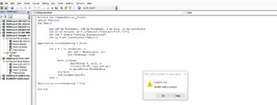
Specifically, I need to know how to automatically copy negative numbers from the original source sheet into a second sheet, and positive numbers into a third sheet. For clarity, I download daily bank transactions with many lines, and I figured there has to be a simpler way to do this rather than copying and pasting a lot of data. I need help having one sheet pull the posting date, reference, amount and class into a Debits sheet (negative numbers) and Credits sheet (positive). I'm assuming an advanced filter should be used, but I don't have unique data for this to easily occur. Shouldn't a sheet be able to look up a range of another, read it, and copy the specific criteria I'm seeking? I'm sorry if this still doesn't make sense. I've included a sample sheet of raw data from downloaded statements. Ideally, the Debits and Credits sheets should automatically update/refresh -- or at least do so with the click of a macro button-- each time I add new data to an existing table.

Sample Stmt Download.xlsx
	E	F	G	H	I	J	K	L
1	Post Date	Reference	Additional Reference	Amount	Description	Type	Class	Text
2	6/1/2022	GE		$29,166.67	INCOMING WIRE TRANSFER	Wire	Miscellaneous Deposit	GU
3	6/1/2022	UKOGF FOUNDATION Payments		$3.49	ACH CREDIT	Ach	Development	UKOGF FOUNDATION Payments
4	6/1/2022	5/3 BANKCARD SYS COMB. DEP.		$275.50	ACH CREDIT	Ach	Bookstore	5/3 BANKCARD SYS COMB. DEP. Worldpay
5	6/1/2022	Virginia529 EDI PYMNTS		$2,167.42	ACH CREDIT	Ach	Tuition	Virginia529 EDI PYMNTS
6	6/1/2022	5335	5335	($2,290.99)	CHECK PAID	Check	Check
7	6/1/2022	60122152	60122152	($39,234.49)	LOAN PAYMENT	Loan	Loan	847,,AUTOMATIC LOAN PAY
8	6/2/2022	Square Inc 220602P2		$48.25	ACH CREDIT	Ach	Eagles' Wings	Square Inc Bird Wings
9	6/2/2022	Virginia529 EDI PYMNTS		$1,100.00	ACH CREDIT	Ach	Tuition	Virginia529 EDI PYMNTS
10	6/2/2022	SEMI MONTHLY FSA TRA		($3,957.60)	MISC. DEBIT	Transfer	FSA	SEMI MONTHLY FSA TRANSFER
11	6/2/2022	WWEX Franchise H EP		($277.54)	PREAUTHORIZED ACH DEBIT	Ach	WWEx	WWEX Franchise
12	6/3/2022			$103.46	DEPOSIT	Deposit	Deposit
13	6/3/2022	3257-22 BB Merchan		$67.66	ACH CREDIT	Ach	BBMS	3257-22 BB Merchan
14	6/3/2022	AVIDPAY SERVICE AV		($15.05)	PREAUTHORIZED ACH DEBIT	Ach	AvidPay ACH	AVIDPAY SERVICE AVIDPAY
15	6/3/2022	GONZAGA COLLEGE MO		($19,600.00)	PREAUTHORIZED ACH DEBIT	Ach	ACH	GCHS
16	6/3/2022	Voya Nat Trst182 SP		($88,409.72)	PREAUTHORIZED ACH DEBIT	Ach	Payroll	Voya Nat Trst182
17	6/6/2022	ACTIVE NETWORK, REGISTRATI		$50,669.64	ACH CREDIT	Ach	Active Network	ACTIVE NETWORK,
18	6/7/2022	MERCHANTSERVCS BI		($29.99)	PREAUTHORIZED ACH DEBIT	Ach	Bank Fees	MERCHANTSERVCS BILLNG School Store
19	6/17/2022	Square Inc 220617P2		$48.25	ACH CREDIT	Ach	Square Deposit	Square Inc BirdWings
20	6/17/2022	SMART LLC SMART LLC		$37,287.31	ACH CREDIT	Ach	Smart Tuition	SMART LLC SMART LLC
06-2022 Daily Transactions

 

[My Aswer Is This]

So, if I understand if the value in column H is positive copy this row to a sheet named Positive
And if the value in column H is negative copy this row to a sheet named Negative
But only copy the values in Column E, F, H and K
Is this correct?

If not give me all 3 sheet names.
And how do you expect to activate the script?
By clicking a button and copy all the rows in your sheet at the same time that meet the criteria?
Or when you double click on a cell in the row or enter a value in a cell on the sheet.
Please be specific with all your answers.
Say When I double click or enter a specific value in column G
Specifics are always important
And when we copy parts of this row to the other sheet do we delete the row from the original sheet?

 

[NewFrugal]

So, if I understand if the value in column H is positive copy this row to a sheet named Positive
And if the value in column H is negative copy this row to a sheet named Negative
But only copy the values in Column E, F, H and K
Is this correct?

If not give me all 3 sheet names.
And how do you expect to activate the script?
By clicking a button and copy all the rows in your sheet at the same time that meet the criteria?
Or when you double click on a cell in the row or enter a value in a cell on the sheet.
Please be specific with all your answers.
Say When I double click or enter a specific value in column G
Specifics are always important
And when we copy parts of this row to the other sheet do we delete the row from the original sheet?

Hello. You're on the right track. Here's more clarification:

Yes, if the value in column H is positive, copy the row to a sheet named Credits. If the value in column H is negative, its respective row would copy to a sheet named Debits. The original source sheet/tab is named 06-2022 Transactions.

Values in columns E through K would need to be copied (E, F, G, H, I, J, and K). Essentially, it would be the entire row, but I hid columns A-D because the info is immaterial and inconsequential.

As far as activating the script, pardon my ignorance, but do you mean via VBA/macros?
I'd like both the Credits and Debits sheets to have Refresh buttons, so that after I've entered new data (new lines) into the table on the original source sheet (06-2022 Transactions), I can go to those respective sheets, click their Refresh buttons, and the new entries will automatically appear based on column H's value.

No, nothing should be deleted from the original sheet when rows are copied to the new sheets. I have to retain original source information for audit purposes.

Please let me know if I'm lacking specifics. Thank you for taking the time to respond to my inquiry. I sincerely appreciate your time and assistance!

 

[My Aswer Is This]

You said:
As far as activating the script, pardon my ignorance, but do you mean via VBA/macros?
Sure, this must be done using a vba script.

And you said Refresh Button.
I do not know what a refresh button is.
I have been using Excel for years but do not know what you mean by refresh button.
Or do you mean when you click on a Button to run a script

And I asked:
And how do you expect to activate the script?
By clicking a button and copy all the rows in your sheet at the same time that meet the criteria?
Or when you double click on a cell in the row or enter a value in a cell on the sheet to copy just that row.

 

[NewFrugal]

You said:
As far as activating the script, pardon my ignorance, but do you mean via VBA/macros?
Sure, this must be done using a vba script.

And you said Refresh Button.
I do not know what a refresh button is.
I have been using Excel for years but do not know what you mean by refresh button.
Or do you mean when you click on a Button to run a script

And I asked:
And how do you expect to activate the script?
By clicking a button and copy all the rows in your sheet at the same time that meet the criteria?
Or when you double click on a cell in the row or enter a value in a cell on the sheet to copy just that row.

Thank you for your patience.

You're correct in regards to a Refresh button. In essence, a refresh button is simply a reload button to reload the page with updated data. In this case, the button name would simply be Refresh (instead of something like "Click Here" or "Reload"). When this button is clicked, it should run a script that pulls all the rows that meet criteria for the specific sheet (sheet named Credits pulls all rows with positive values in column H; sheet named Debits pulls all rows with negative values in column). Nothing from the original source sheet should be deleted as information is pulled into the other sheets. The best way I can put it is that the workbook should function similar to an advanced filter with automatic updates based on new information that is keyed in daily since I download bank transactions daily.

 

[vcoolio]

Hello NewFrugal,

Assuming that your data is in an actual, formal Excel table, here's one option using only one button on the main sheet:-

Option Explicit
Sub Test()

        Dim wsT As Worksheet, wsD As Worksheet, i As Long
        Dim ar As Variant: ar = [{"Debits","Credits";"<0",">0"}]
        Set wsT = Sheets("06-2022 Transactions")
        
Application.ScreenUpdating = False

        For i = 1 To UBound(ar, 2)
                     Set wsD = Sheets(ar(1, i))
                     wsD.UsedRange.Clear
                    
              With wsT.ListObjects("Table2").Range '---->Change table name to suit
                      .AutoFilter 8, ar(2, i)
                      .Columns("E:K").Copy wsD.[A1]
              End With
                      If wsT.FilterMode = True Then
                            wsT.ShowAllData
                      End If
              wsD.Columns.AutoFit
        Next i

Application.ScreenUpdating = True

End Sub

You'll just need to change the table name to suit. Assign the code to a button on your main sheet.
Please test the code in a copy of your actual workbook first.

I hope that this helps.

Cheerio,
vcoolio.

 

[vcoolio]

Hello NewFrugal,

I've just changed the above code a little as the ShowAllData line may possibly error. The updated code is as follows:-

Option Explicit
Sub Test()

        Dim wsT As Worksheet, wsD As Worksheet, i As Long, lo As ListObject
        Dim ar As Variant: ar = [{"Debits","Credits";"<0",">0"}]
        Set wsT = Sheets("06-2022 Transactions")
        Set lo = wsT.ListObjects("Table2") '---->Change table name to suit.
        
Application.ScreenUpdating = False

        For i = 1 To UBound(ar, 2)
                     Set wsD = Sheets(ar(1, i))
                     wsD.UsedRange.Clear
                    
              With lo.Range
                      .AutoFilter 8, ar(2, i)
                      .Columns("E:K").Copy wsD.[A1]
                      lo.AutoFilter.ShowAllData
              End With
              wsD.Columns.AutoFit
        Next i

Application.ScreenUpdating = True

End Sub

I've also declared a variable this time for the Listobject (Table2).

Cheerio,
vcoolio.

 

[NewFrugal]

Hello NewFrugal,

I've just changed the above code a little as the ShowAllData line may possibly error. The updated code is as follows:-

Option Explicit
Sub Test()

        Dim wsT As Worksheet, wsD As Worksheet, i As Long, lo As ListObject
        Dim ar As Variant: ar = [{"Debits","Credits";"<0",">0"}]
        Set wsT = Sheets("06-2022 Transactions")
        Set lo = wsT.ListObjects("Table2") '---->Change table name to suit.
       
Application.ScreenUpdating = False

        For i = 1 To UBound(ar, 2)
                     Set wsD = Sheets(ar(1, i))
                     wsD.UsedRange.Clear
                   
              With lo.Range
                      .AutoFilter 8, ar(2, i)
                      .Columns("E:K").Copy wsD.[A1]
                      lo.AutoFilter.ShowAllData
              End With
              wsD.Columns.AutoFit
        Next i

Application.ScreenUpdating = True

End Sub

I've also declared a variable this time for the Listobject (Table2).

Cheerio,
vcoolio.

Hi, vcoolio. Thank you for responding. I tried assigning the code you provided to a button, but the Visual Basic editor keeps returning an error message. Please see the attached image. I don't really know what I'm doing when it comes to assigning the code to a button, but I've been under Design Mode trying to use an ActiveX control button.

 

[NewFrugal]

Hello NewFrugal,

I've just changed the above code a little as the ShowAllData line may possibly error. The updated code is as follows:-

Option Explicit
Sub Test()

        Dim wsT As Worksheet, wsD As Worksheet, i As Long, lo As ListObject
        Dim ar As Variant: ar = [{"Debits","Credits";"<0",">0"}]
        Set wsT = Sheets("06-2022 Transactions")
        Set lo = wsT.ListObjects("Table2") '---->Change table name to suit.
       
Application.ScreenUpdating = False

        For i = 1 To UBound(ar, 2)
                     Set wsD = Sheets(ar(1, i))
                     wsD.UsedRange.Clear
                   
              With lo.Range
                      .AutoFilter 8, ar(2, i)
                      .Columns("E:K").Copy wsD.[A1]
                      lo.AutoFilter.ShowAllData
              End With
              wsD.Columns.AutoFit
        Next i

Application.ScreenUpdating = True

End Sub

I've also declared a variable this time for the Listobject (Table2).

Cheerio,
vcoolio.

You can disregard my last message to you. I figured out what I did wrong, and the coding now works. Thank you so much for your help!

 

[vcoolio]

You're welcome NewFrugal. I'm glad to have been able to assist.

Cheerio,
vcoolio.