Rank duplicate numbers

[ORoxo]

Hello again, guys
I'm using the following formula to rank Risks according to the value in a cell. However, right now, the formula ignores duplicates.

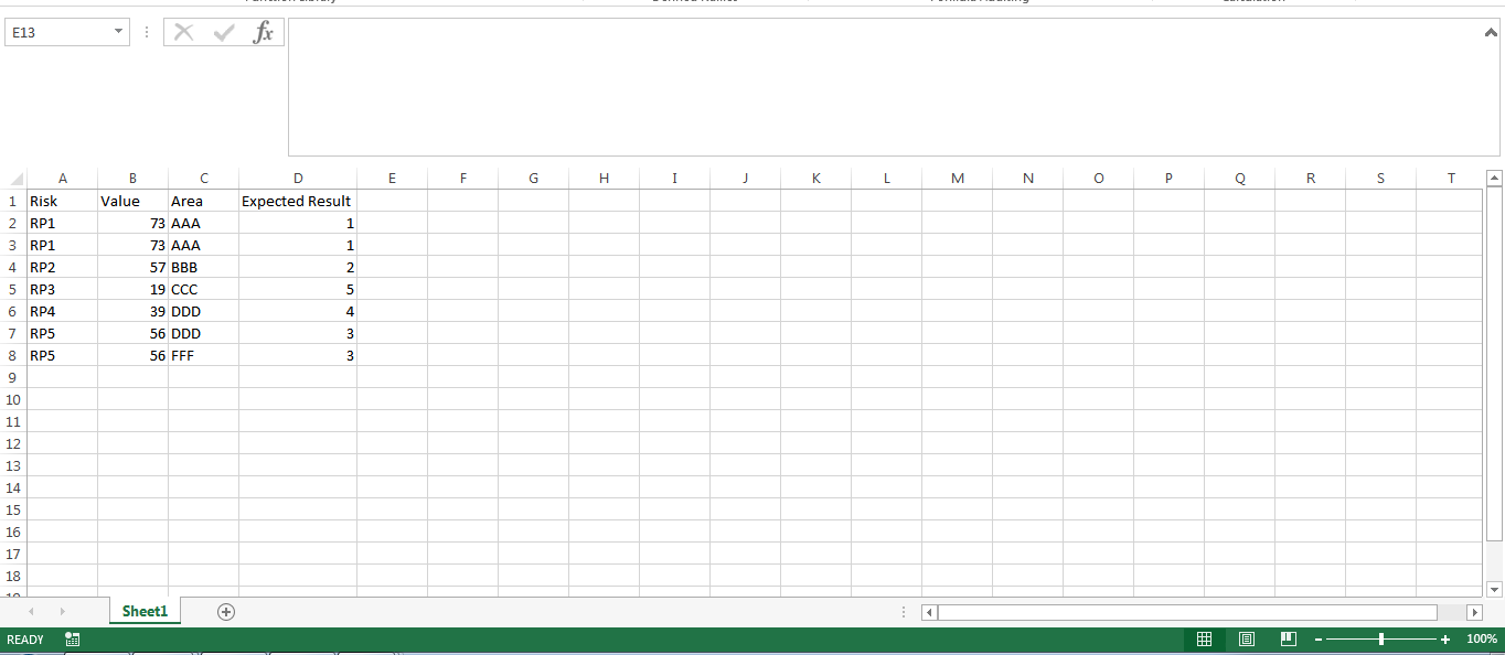
Let's say I have the same risk listed twice - which can happen. The formula will just ignore this and assign it the next available number. I was hoping there's some way for it take into consideration the previous number assigned to a specific risk.
This is a sample and the expected result:

Thanks!

 

[Eric W]

Maybe:

	A	B	C	D	E
1	Risk	Value	Area	Expected Result
2	RP1	73	AAA	1
3	RP1	73	AAA	1
4	RP2	57	BBB	2
5	RP3	19	CCC	5
6	RP4	39	DDD	4
7	RP5	56	DDD	3

<tbody>
</tbody>

Sheet5​

Array Formulas Cell Formula D2 {=SUM(SIGN(FREQUENCY(IF($B$2:$B$8>B2,MATCH($A$2:$A$8,$A$2:$A$8,0)),ROW($A$2:$A$8)-ROW($A$2)+1)))+1} <tbody> </tbody> Entered with Ctrl+Shift+Enter. If entered correctly, Excel will surround with curly braces {}. Note: Do not try and enter the {} manually yourself

<tbody>
</tbody>

 

[ORoxo]

Maybe:

	A	B	C	D	E
1	Risk	Value	Area	Expected Result
2	RP1	73	AAA	1
3	RP1	73	AAA	1
4	RP2	57	BBB	2
5	RP3	19	CCC	5
6	RP4	39	DDD	4
7	RP5	56	DDD	3

<tbody>
</tbody>

Sheet5​

Array Formulas Cell Formula D2 {=SUM(SIGN(FREQUENCY(IF($B$2:$B$8>B2,MATCH($A$2:$A$8,$A$2:$A$8,0)),ROW($A$2:$A$8)-ROW($A$2)+1)))+1} <tbody> </tbody> Entered with Ctrl+Shift+Enter. If entered correctly, Excel will surround with curly braces {}. Note: Do not try and enter the {} manually yourself

<tbody>
</tbody>

This is not exactly what I am looking for although it works for that sample, I'm sorry. I will try to make use of a better example:

Risk	Value	Department	Expected Value
RA11	22	A&T	1
RA11	22	A&T	1
RA44	22	A&T	2
RA45	22	A&T	3
RA46	22	A&T	4
RC8	27,5	COM	1
RC8	27,5	COM	1
RC8	27,5	COM	1
RC8	27,5	COM	1
RC34	22	COM	2

<tbody>
</tbody>

Basically, I would like the formula to have into consideration department and the number of the risk. It should rank same for the same risk, regardless of how many times it appears and it should rank them at a department level only.

Thanks once again for the support

 

[Eric W]

Try:

Excel 2012

	A	B	C	D
1	Risk	Value	Department	Expected Value
2	RA11	22	A&T	1
3	RA11	22	A&T	1
4	RA44	22	A&T	2
5	RA45	22	A&T	3
6	RA46	22	A&T	4
7	RC8	27,5	COM	1
8	RC8	27,5	COM	1
9	RC8	27,5	COM	1
10	RC8	27,5	COM	1
11	RC34	22	COM	2

<colgroup><col style="width: 25pxpx"><col><col><col><col></colgroup><thead>
</thead><tbody>
</tbody>

Sheet1​

Array Formulas Cell Formula D2 {=SUM(SIGN(FREQUENCY(IF($C$2:$C$11=C2,IF(MID($A$2:$A$11,3,9)+0<MID(A2,3,9)+0,MATCH($A$2:$A$11,$A$2:$A$11,0))),ROW($A$2:$A$11)-ROW($A$2)+1)))+1} <thead> </thead><tbody> </tbody> Entered with Ctrl+Shift+Enter. If entered correctly, Excel will surround with curly braces {}. Note: Do not try and enter the {} manually yourself

<tbody>
</tbody>

Using column A for the rating is a bit problematic. I assumed that there is a 2-character prefix, and then the rest of the value is the rating.

 

[ORoxo]

Try:

Excel 2012

	A	B	C	D
1	Risk	Value	Department	Expected Value
2	RA11	22	A&T	1
3	RA11	22	A&T	1
4	RA44	22	A&T	2
5	RA45	22	A&T	3
6	RA46	22	A&T	4
7	RC8	27,5	COM	1
8	RC8	27,5	COM	1
9	RC8	27,5	COM	1
10	RC8	27,5	COM	1
11	RC34	22	COM	2

<tbody>
</tbody>

Sheet1​

Array Formulas Cell Formula D2 {=SUM(SIGN(FREQUENCY(IF($C$2:$C$11=C2,IF(MID($A$2:$A$11,3,9)+0<mid(<font color="#FF00FF">A2</mid(<font color="Blue"><font color="Red"><mid(,3,9</mid()+0,MATCH($A$2:$A$11,$A$2:$A$11,0))),ROW($A$2:$A$11)-ROW($A$2)+1)))+1} <tbody> </tbody> Entered with Ctrl+Shift+Enter. If entered correctly, Excel will surround with curly braces {}. Note: Do not try and enter the {} manually yourself

<tbody>
</tbody>

Using column A for the rating is a bit problematic. I assumed that there is a 2-character prefix, and then the rest of the value is the rating.

Eric, thanks again fr your help! Could you please check the part in red bold on your formula?

Thanks

 

[Eric W]

Ugh! Sorry, I still get caught occasionally by a quirk where the forum interprets a < as an HTML tag and not as an operator:

=SUM(SIGN(FREQUENCY(IF($C$2:$C$11=C2,IF(MID($A$2:$A$11,3,9)+0< MID(A2,3,9)+0,MATCH($A$2:$A$11,$A$2:$A$11,0))),ROW($A$2:$A$11)-ROW($A$2)+1)))+1

 

[ORoxo]

Ugh! Sorry, I still get caught occasionally by a quirk where the forum interprets a < as an HTML tag and not as an operator:

=SUM(SIGN(FREQUENCY(IF($C$2:$C$11=C2,IF(MID($A$2:$A$11,3,9)+0< MID(A2,3,9)+0,MATCH($A$2:$A$11,$A$2:$A$11,0))),ROW($A$2:$A$11)-ROW($A$2)+1)))+1

Thanks, Eric! This does work perfectly. I would just like it to take int consideration column B. Would that be possible?

 

[Eric W]

In what way do you want to consider column B? As part of the rating (if so, how), or as part of the department grouping (again, if so, how)?

 

[ORoxo]

In what way do you want to consider column B? As part of the rating (if so, how), or as part of the department grouping (again, if so, how)?

I want it to consider it as part of the ranking.

In other words, I want to rank the risks according to the value in column B and within each department, that's the general rule. Let's say, however, that I have two rows in my dataset with the same Risk Name. In that case, I want it to give it the same rank.

If it's not yet clear let me know, I will try to explain it in another way.

 

[Eric W]

I don't think I quite picture it. Could you post an example? And could you verify that the risk ranking is based on column A, without the first 2 characters?