Ranking Data Based on Multiple Criteria

[sethk1024]

As the title suggests, I'm looking to use the RANK function in excel, however, I'd like to rank given samples of data within multiple criteria.

I've attached an abbreviated sample of a much larger data set in the image here.

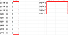
In the first table on the left...

I have 3 NFL football players mentioned, with 4 weeks of points scored in each of 2 seasons, 2019 and 2020. For the sake of this data, lets assume 4 weeks of scoring in a given year constitutes a "full season" for that player.

The primary thing I'd like to do here is rank the points scored based on:
- the player who scored the points
- the week the points are scored in
- the year the points are scored in

So, for example, Aaron Rodgers in Week 1 of 2019 scored 29 points. Amongst other players who played in Week 1 of 2019 in this dataset, that score of 29 points ranks first.

I'd like to rank all scores of all weeks in all years in a similar manner.


Then, using that data, I'd like to create a separate rank (in the table on the right) which sums up all the points scored for all the weeks in a given year, and ranks that sum amongst other players who played in a given season. This again is based on:
- the player who scored the points
- all weeks the points are scored in a given season
- the year the points are scored in

So, for example, Aaron Rodgers had 81 points in 4 games played in 2019, which ranks second amongst the three players in this dataset.

I'd like to do this ranking for each year of data for a given player, as well as the average of all years of data.

So, for example, taking the average of all points Aaron Rodgers scored in 2019, and 2020 (all available data points for a given player in the large dataset for points scored), he finished with the second most points amongst the three players mentioned.


Lastly, I'd like to rank the average weekly finish.

So, for example, when averaging the weekly finishes (lowest rank = most points in a given week) of Aaron Rodgers in 2019, Aaron Rodgers finished second, meaning, he finished as the highest ranked QB, on average, second most often. I would like to rank this based on the same criteria as the above when we calculated the yearly point total ranks.



I know this is a lengthy post without various calculations and is probably worded a bit poorly and confusing! If there's anything I can do to simplify the post and clarify any confusion, please let me know. Thank you very much and I appreciate the help!!

 

[bebo021999]

It requires 2 helpers columns for the right table

Book1
	A	B	C	D	E	F	G	H	I	J	K	L	M	N	O
1	Player	Year	Week	Points	WeeklyFinishes					Player	Year	Yearly Total Points Rank	Rank of Average Weekly Finishes	Yearly Total Points	Average Weekly Finishes
2	AA	2019	1	29	1					AA	2019	3	2	81	2.25
3	AA	2019	2	16	3					BB	2019	1	1	120	1.25
4	AA	2019	3	21	2					CC	2019	2	3	94	2.50
5	AA	2019	4	15	3					AA	2020	3	2	95	2.00
6	AA	2020	1	29	1					BB	2020	1	1	106	1.75
7	AA	2020	2	19	2					CC	2020	2	3	96	2.25
8	AA	2020	3	23	2					AA	All	3	2	176	2.13
9	AA	2020	4	24	3					BB	All	1	1	226	1.50
10	BB	2019	1	28	2					CC	All	2	3	190	2.38
11	BB	2019	2	33	1
12	BB	2019	3	23	1
13	BB	2019	4	36	1
14	BB	2020	1	26	2									Helper Columns
15	BB	2020	2	17	3
16	BB	2020	3	26	1
17	BB	2020	4	37	1
18	CC	2019	1	24	3
19	CC	2019	2	17	2
20	CC	2019	3	19	3
21	CC	2019	4	34	2
22	CC	2020	1	16	3
23	CC	2020	2	28	1
24	CC	2020	3	20	3
25	CC	2020	4	32	2
Sheet1

Cell Formulas
Range	Formula
L2:L10	L2	=COUNTIFS($K$2:$K$10,K2,$N$2:$N$10,">=" &N2)
M2:M10	M2	=COUNTIFS($K$2:$K$10,K2,$O$2:$O$10,"<=" &O2)
N2:N10	N2	=IF(K2="All",SUMIFS($D$2:$D$25,$A$2:$A$25,J2),SUMIFS($D$2:$D$25,$A$2:$A$25,J2,$B$2:$B$25,K2))
O2:O10	O2	=IF(K2="All",AVERAGEIFS($E$2:$E$25,$A$2:$A$25,J2),AVERAGEIFS($E$2:$E$25,$A$2:$A$25,J2,$B$2:$B$25,K2))
E2:E25	E2	=COUNTIFS($B$2:$B$25,B2,$C$2:$C$25,C2,$D$2:$D$25,">=" & D2)

 

[sethk1024]

It requires 2 helpers columns for the right table

Book1
	A	B	C	D	E	F	G	H	I	J	K	L	M	N	O
1	Player	Year	Week	Points	WeeklyFinishes					Player	Year	Yearly Total Points Rank	Rank of Average Weekly Finishes	Yearly Total Points	Average Weekly Finishes
2	AA	2019	1	29	1					AA	2019	3	2	81	2.25
3	AA	2019	2	16	3					BB	2019	1	1	120	1.25
4	AA	2019	3	21	2					CC	2019	2	3	94	2.50
5	AA	2019	4	15	3					AA	2020	3	2	95	2.00
6	AA	2020	1	29	1					BB	2020	1	1	106	1.75
7	AA	2020	2	19	2					CC	2020	2	3	96	2.25
8	AA	2020	3	23	2					AA	All	3	2	176	2.13
9	AA	2020	4	24	3					BB	All	1	1	226	1.50
10	BB	2019	1	28	2					CC	All	2	3	190	2.38
11	BB	2019	2	33	1
12	BB	2019	3	23	1
13	BB	2019	4	36	1
14	BB	2020	1	26	2									Helper Columns
15	BB	2020	2	17	3
16	BB	2020	3	26	1
17	BB	2020	4	37	1
18	CC	2019	1	24	3
19	CC	2019	2	17	2
20	CC	2019	3	19	3
21	CC	2019	4	34	2
22	CC	2020	1	16	3
23	CC	2020	2	28	1
24	CC	2020	3	20	3
25	CC	2020	4	32	2
Sheet1

Cell Formulas
Range	Formula
L2:L10	L2	=COUNTIFS($K$2:$K$10,K2,$N$2:$N$10,">=" &N2)
M2:M10	M2	=COUNTIFS($K$2:$K$10,K2,$O$2:$O$10,"<=" &O2)
N2:N10	N2	=IF(K2="All",SUMIFS($D$2:$D$25,$A$2:$A$25,J2),SUMIFS($D$2:$D$25,$A$2:$A$25,J2,$B$2:$B$25,K2))
O2:O10	O2	=IF(K2="All",AVERAGEIFS($E$2:$E$25,$A$2:$A$25,J2),AVERAGEIFS($E$2:$E$25,$A$2:$A$25,J2,$B$2:$B$25,K2))
E2:E25	E2	=COUNTIFS($B$2:$B$25,B2,$C$2:$C$25,C2,$D$2:$D$25,">=" & D2)

sorry for the slow reply. ive been playing around with a bunch of stuff and trying to understand everything you wrote out in the sheet.

*thank you so much* – this is exactly what I needed. extremely helpful!

 

[sethk1024]

It requires 2 helpers columns for the right table

Book1
	A	B	C	D	E	F	G	H	I	J	K	L	M	N	O
1	Player	Year	Week	Points	WeeklyFinishes					Player	Year	Yearly Total Points Rank	Rank of Average Weekly Finishes	Yearly Total Points	Average Weekly Finishes
2	AA	2019	1	29	1					AA	2019	3	2	81	2.25
3	AA	2019	2	16	3					BB	2019	1	1	120	1.25
4	AA	2019	3	21	2					CC	2019	2	3	94	2.50
5	AA	2019	4	15	3					AA	2020	3	2	95	2.00
6	AA	2020	1	29	1					BB	2020	1	1	106	1.75
7	AA	2020	2	19	2					CC	2020	2	3	96	2.25
8	AA	2020	3	23	2					AA	All	3	2	176	2.13
9	AA	2020	4	24	3					BB	All	1	1	226	1.50
10	BB	2019	1	28	2					CC	All	2	3	190	2.38
11	BB	2019	2	33	1
12	BB	2019	3	23	1
13	BB	2019	4	36	1
14	BB	2020	1	26	2									Helper Columns
15	BB	2020	2	17	3
16	BB	2020	3	26	1
17	BB	2020	4	37	1
18	CC	2019	1	24	3
19	CC	2019	2	17	2
20	CC	2019	3	19	3
21	CC	2019	4	34	2
22	CC	2020	1	16	3
23	CC	2020	2	28	1
24	CC	2020	3	20	3
25	CC	2020	4	32	2
Sheet1

Cell Formulas
Range	Formula
L2:L10	L2	=COUNTIFS($K$2:$K$10,K2,$N$2:$N$10,">=" &N2)
M2:M10	M2	=COUNTIFS($K$2:$K$10,K2,$O$2:$O$10,"<=" &O2)
N2:N10	N2	=IF(K2="All",SUMIFS($D$2:$D$25,$A$2:$A$25,J2),SUMIFS($D$2:$D$25,$A$2:$A$25,J2,$B$2:$B$25,K2))
O2:O10	O2	=IF(K2="All",AVERAGEIFS($E$2:$E$25,$A$2:$A$25,J2),AVERAGEIFS($E$2:$E$25,$A$2:$A$25,J2,$B$2:$B$25,K2))
E2:E25	E2	=COUNTIFS($B$2:$B$25,B2,$C$2:$C$25,C2,$D$2:$D$25,">=" & D2)

Hey thanks again. I've been playing around with this trying to implement in my sheet , however, i noticed a shortcoming in the solution you provided.

It only works as you coded it because, for example, if i want to rank the yearly total points, it uses the helper column to the right of the table, which only has 10 rows.

but i realized if i add new players to the dataset, it no longer works. i have thousands of cells for a given player pool, so to copy the cells over and over would get messy. know what I mean?

is there another solution, maybe something I can add to the original table that would allow me to reference the original data without needing ALL of that data in the helper table?

what i mean is...

the original data set has THOUSANDS of players in the ranking.

however, my final table only has a small fraction of those players.

having to have a table with all of the players would be both cumbersome, and useless for my end goal.

if you need more clarification, i will gladly provide it. not sure if my issue is making sense?

 

[bebo021999]

With thousand players, VBA should be a good choice.
Is it acceptable?
Try to attch a mini sheet via XL2BB.

XL2BB - Excel Range to BBCode

Excel 'mini-sheet' in messages - XL2BB Although experts prefer to read your description and question instead of working in your actual file to solve your problem, there are times that it is difficult to explain an issue without providing actual...

www.mrexcel.com