Ranking sales and group in 5 tier's VBA or Macro help

jlhop66

New Member
Joined
Apr 24, 2014
Messages
10
Office Version
  1. 365
Platform
  1. Windows
Hello Group!!! I am working with a very large data set of 200+ items across 3,000+ stores. I finally figured out the equation to rank stores by sales velocity, and an equation to put the stores into 5 groups of stores for analysis. right now I am doing this manually and it takes me 7 to 9 hours each week, this is killing me.

my challenge is creating a VBA program to run my equations for the length of store numbers that vary from 600 to 3,00 stores and start over at the next item number in the list. I need to make this program to loop over and over until it reached the end of the item number list witch is in column "A".

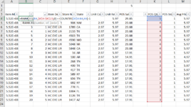
Rank store sales: 1 through 600 or 3,000 (store count vary) (Column "K" is my sales qty)
This data is in Column "B" - FYI, I can put this data at the end of my data table if that makes it easier.
=RANK.EQ(K10,$K$10:$K$2598,0)+COUNTIF($K10:K10,K10)-1

This data is in Column "C"
Grouping of ranked stores - FYI, I can also put this data at the end of my data table if that makes it easier.
=MAX( ROUNDUP( PERCENTRANK($B$10:$B$2929, B10) *$I$1, 0),1)


Here is my attempt to write the VBA code - but it's not work. any help is greatly appreciated.

Sub aTest()
Dim LR As Long, rCell As Range, strAdd As String

LR = Cells(Rows.Count, "K").End(xlUp).Row
With Range("K4:K" & LR)
.Formula = "=RANK.EQ(K4,$K$4:$K$2592,0)+COUNTIF($K4:K4,K4)-1))"
.NumberFormat = "0%"
End With

For Each rCell In Range("B4:B" & LR)
If rCell <> "" Then
strAdd = rCell.Address
Else
rCell.Formula = MAX( ROUNDUP( PERCENTRANK($B$4:$B$2923, B4) *$I$1, 0),1)
End If
Next rCell
End Sub

Column "B" equation example
1658164570396.png


Column "C" equation example
1658164665663.png
 

Excel Facts

Test for Multiple Conditions in IF?
Use AND(test, test, test, test) or OR(test, test, test, ...) as the logical_test argument of IF.
Hi,

you could try this to see if it works. The loop inserts both formulas into their respective columns with each pass. I learned his kind of approach from FLUFF on here just few days ago.. so big shoutout to him.
Rob

VBA Code:
Sub Rank()
   Dim Rng As Range
   
   lastrow = ActiveSheet.Cells(Rows.Count, 1).End(xlUp).Row
   
   For Each Rng In Range("A4", Range("A" & Rows.Count).End(xlUp))
       
      Rng.Offset(0, 1).Resize(Rng.Count).FormulaR1C1 = "=RANK.EQ(R[0]C11,R4C11:R" & lastrow & "C11,0) + COUNTIF(R[0]C11:R[0]C11,R[0]C11)-1"
      
      Rng.Offset(0, 2).Resize(Rng.Count).FormulaR1C1 = "=MAX(ROUNDUP(PERCENTRANK(R4C2:R" & lastrow & "C2,R[0]C2)*R1C9,0),1)"
      
   Next Rng
   
End Sub
 
Upvote 0
Wow, it almost worked perfectly and I am grateful to get this far. I still think I messed something up because the cells are not locking in the correct columns. I think I originally put the "$" symbols in the wrong place or something. the loop is working perfectly, but my equations are not wrong or something.

in the small sample store list below, I corrected the equations after the VBA ran and I get the ranking correct and the groupings to work 1 through 5. So I know i am doing something wrong with the equation or something.

Rng.Offset(0, 1).Resize(Rng.Count).FormulaR1C1 = "=RANK.EQ(R[0]C11,R4C11:R" & lastrow & "C11,0) + COUNTIF(R[0]C11:R[0]C11,R[0]C11)-1"

Rng.Offset(0, 2).Resize(Rng.Count).FormulaR1C1 = "=MAX(ROUNDUP(PERCENTRANK(R4C2:R" & lastrow & "C2,R[0]C2)*R1C9,0),1)"

=RANK.EQ(J4,$J$4:$J$23,0) + COUNTIF($J$4:J4,J4)-1
1658272867246.png


=MAX(ROUNDUP(PERCENTRANK($B$4:$B$23,B4)*$I$1,0),1)
1658272601991.png
 

Attachments

  • 1658272533359.png
    1658272533359.png
    65.9 KB · Views: 8
Upvote 0
Hi,

So I can see the problem is that you removed a column (Category?) in your data from the initial posting versus your reply yesterday - and that means the formula being inserted by the macro is referencing the wrong column.

Here's the update for you. I've also used the $ signs in the way you want them in your formula just so your comfortable, but really it doesn't affect the way the formula works on its particular row in this instance versus the original code.

Looking further, I played also with removing the +COUNTIF statement, as I can't see what this is doing for you ? Just using the Rank alone is Ranking the items in order correctly versus your POS Qty ? You can remove it therefore as far as I can see.

For your second formula, I confess to not understand what you are trying to achieve with it (I couldn't see what the groups were supposed to be) - but as long as your happy with your formulas then all should be good.

Let me know how you get on.

VBA Code:
Sub Rank()
   Dim Rng As Range
   
   lastrow = ActiveSheet.Cells(Rows.Count, 1).End(xlUp).Row
   
   For Each Rng In Range("A4", Range("A" & Rows.Count).End(xlUp))
       
      Rng.Offset(0, 1).FormulaR1C1 = "=RANK.EQ(R[0]C10,R4C10:R" & lastrow & "C10,0) + COUNTIF(R[0]C10:R[0]C10,R[0]C[8])-1"
      
      Rng.Offset(0, 2).FormulaR1C1 = "=MAX(ROUNDUP(PERCENTRANK(R4C2:R" & lastrow & "C2,R[0]C[-1])*R1C9,0),1)"
      
   Next Rng
   
End Sub
 
Upvote 0
I am getting closer. below I have updated my VBA code so that Column B is ranking the Sales column in "J" highest to lowest. the code is saying last row, but I need to stop at the change in item number in column "A" and start the ranking over again until it finds a change in item number in column "A" again, and so on down the sheet till it runs out of item number. below i have more examples of what the result are. thank you very much.

VBA Code
Sub Demo_3_test()
Dim Rng As Range

lastrow = ActiveSheet.Cells(Rows.Count, 1).End(xlUp).Row

For Each Rng In Range("A4", Range("A" & Rows.Count).End(xlUp))

Rng.Offset(0, 1).FormulaR1C1 = "=RANK.EQ(R[0]C[8],R4C10:R" & lastrow & "C10,0) + COUNTIF(R[0]C[10]:R4C10,R[0]C[8])-1"

Rng.Offset(0, 2).FormulaR1C1 = "=MAX(ROUNDUP(PERCENTRANK(R4C2:R" & lastrow & "C2,R[0]C[-1])*R1C9,0),1)"

Next Rng

End Sub

this is me, manually correcting the Last row to "$J$23" to make the ranking work
1658528361650.png


here at row 24, the VBA code changed my range cells to larger range than it should be.
1658528535825.png
 
Upvote 0
@jlhop66
Could you post a sample data as a table instead of image? So we can copy-paste it to Excel.
Please use XL2BB tool: XL2BB
here at row 24, the VBA code changed my range cells to larger range than it should be.
What the formula in B5 & C5 and B24 & C24 should look like?
 
Upvote 0
Top Store Sales by Item demo.xlsm
ABCDEFGHIJKLMN
15
2
3Item NbrStore RankGroupItem Desc 1Store NbrStateUnit CostUnit RetailPOS SalesPOS QtyPOS Store CountAvg PriceUnits per Store per Week (w/o zeros)Avg Instock %
46255199730511HC EYE LIMIT-758656TN2.975.9717.912215.971.0100%
56255199730521HC EYE LIMIT-758268TN2.975.9717.911815.971.5100%
66255199730531HC EYE LIMIT-7582133TX2.975.9723.881215.972.0100%
76255199730542HC EYE LIMIT-7585048MI2.975.9723.881115.971.30%
86255199730562HC EYE LIMIT-7587294OK2.975.9729.85615.971.3100%
96255199730572HC EYE LIMIT-758906NM2.975.9723.88515.974.00%
106255199730582HC EYE LIMIT-7581789CA2.975.9723.88515.972.0100%
116255199730593HC EYE LIMIT-7584503TX2.975.9723.88415.971.30%
1262551997305103HC EYE LIMIT-7584590MO2.975.9723.88415.974.0100%
1362551997305113HC EYE LIMIT-7585848CA2.975.9723.88415.972.0100%
1462551997305123HC EYE LIMIT-75816AR2.975.9717.91315.973.00%
1562551997305134HC EYE LIMIT-758100AR2.975.9714.91314.971.5100%
1662551997305144HC EYE LIMIT-758400TX2.975.9717.91315.973.0100%
1762551997305154HC EYE LIMIT-758692KY2.975.9717.91315.971.50%
1862551997305164HC EYE LIMIT-758778FL2.975.9717.91315.971.5100%
1962551997305175HC EYE LIMIT-7581417AZ2.975.9717.91315.971.5100%
2062551997305185HC EYE LIMIT-758417TX2.975.9717.91215.971.0100%
2162551997305195HC EYE LIMIT-758589KY2.975.9717.91215.971.5100%
2262551997305205HC EYE LIMIT-7581004FL2.975.9717.91115.971.5100%
236455478043821HC CONTOUR STK-10963294KY$3.57$5.97$2491$5.970.0100%
246455478043811HC CONTOUR STK-10963566CO$3.57$5.97$2491$5.970.0100%
256455478043821HC CONTOUR STK-1096261AR$3.57$5.97$2481$5.970.0100%
266455478043831HC CONTOUR STK-10961888UT$3.57$5.97$2471$5.970.0100%
276455478043841HC CONTOUR STK-10962490KS$3.57$5.97$2471$5.970.00%
286455478043852HC CONTOUR STK-10964627TX$3.57$5.97$2461$5.970.0100%
296455478043862HC CONTOUR STK-10965957CO$3.57$5.97$2451$5.970.0100%
306455478043872HC CONTOUR STK-10961299AZ$3.57$5.97$2451$5.971.00%
316455478043883HC CONTOUR STK-10961785NH$3.57$5.97$2451$5.974.0100%
326455478043893HC CONTOUR STK-1096661AL$3.57$5.97$1841$5.970.0100%
3364554780438103HC CONTOUR STK-10961252CO$3.57$5.97$1841$5.970.00%
3464554780438114HC CONTOUR STK-10961518IN$3.57$5.97$1831$5.970.0100%
3564554780438124HC CONTOUR STK-10961798MI$3.57$5.97$1831$5.970.0100%
3664554780438134HC CONTOUR STK-10961936MI$3.57$5.97$1821$5.970.00%
3764554780438145HC CONTOUR STK-10962086TX$3.57$5.97$1821$5.970.0100%
3864554780438155HC CONTOUR STK-10962206CA$3.57$5.97$1821$5.970.0100%
3964554780438165HC CONTOUR STK-10962496NC$3.57$5.97$1821$5.970.0100%
408259329630011LIP tile-262427TX$3.36$5.97$18161$5.9700.00%
418259329630021LIP tile-261564OH$3.36$5.97$18141$5.971100.00%
428259329630031LIP tile-263783OH$3.36$5.97$18141$5.971100.00%
438259329630041LIP tile-265211TX$3.36$5.97$18141$5.971100.00%
448259329630051LIP tile-26456TX$3.36$5.97$12131$5.9700.00%
458259329630061LIP tile-26789TX$3.36$5.97$12131$5.9700.00%
468259329630071LIP tile-261800TX$3.36$5.97$12121$5.9700.00%
478259329630081LIP tile-262084MT$3.36$5.97$12121$5.9700.00%
488259329630092LIP tile-262910OH$3.36$5.97$12121$5.9700.00%
4982593296300102LIP tile-263478HI$3.36$5.97$13121$6.5700.00%
5082593296300112LIP tile-263897ID$3.36$5.97$12111$5.9700.00%
5182593296300122LIP tile-26304TN$3.36$5.97$12111$5.971100.00%
5282593296300132LIP tile-26467TX$3.36$5.97$12101$5.971100.00%
5382593296300142LIP tile-26664KS$3.36$5.97$12101$5.971100.00%
5482593296300152LIP tile-26848MS$3.36$5.97$12101$5.971100.00%
5582593296300163LIP tile-261113KY$3.36$5.97$12101$5.971100.00%
5682593296300173LIP tile-261253TX$3.36$5.97$1291$5.971100.00%
5782593296300183LIP tile-261663NC$3.36$5.97$1291$5.971100.00%
5882593296300193LIP tile-262222MA$3.36$5.97$1291$5.971100.00%
5982593296300203LIP tile-262423PR$3.36$5.97$1491$7.001100.00%
6082593296300213LIP tile-263270VA$3.36$5.97$1281$5.971100.00%
6182593296300223LIP tile-263827TX$3.36$5.97$1281$5.971100.00%
6282593296300234LIP tile-265350UT$3.36$5.97$1281$5.971100.00%
6382593296300244LIP tile-261185TX$3.36$5.97$1281$5.972100.00%
6482593296300254LIP tile-261231CO$3.36$5.97$1271$5.972100.00%
6582593296300264LIP tile-261370AZ$3.36$5.97$1271$5.972100.00%
6682593296300274LIP tile-261654MN$3.36$5.97$1271$5.972100.00%
6782593296300284LIP tile-263277NV$3.36$5.97$1261$5.972100.00%
6882593296300294LIP tile-263307FL$3.36$5.97$1261$5.972100.00%
6982593296300305LIP tile-264274NC$3.36$5.97$1251$5.972100.00%
7082593296300315LIP tile-264664SC$3.36$5.97$1251$5.972100.00%
7182593296300325LIP tile-264849MN$3.36$5.97$1241$5.972100.00%
7282593296300335LIP tile-26211TX$3.36$5.97$1241$5.973100.00%
7382593296300345LIP tile-26931FL$3.36$5.97$1231$5.973100.00%
7482593296300355LIP tile-262523CA$3.36$5.97$1231$5.973100.00%
7582593296300365LIP tile-265045TX$3.36$5.97$1221$5.973100.00%
7682593296300375LIP tile-622170CT$3.36$5.97$1221$5.974100.00%
Top_Store_Sales_by_Item
Cell Formulas
RangeFormula
B4:B7,B9:B22B4=RANK.EQ(J4,$J$4:$J$23,0) + COUNTIF($J$4:J4,J4)-1
C4:C23C4=MAX(ROUNDUP(PERCENTRANK($B$4:$B$23,B4)*$I$1,0),1)
B8B8=RANK.EQ(J8,$J$4:$J$23,0) + COUNTIF($J5:J$12,J8)-1
B23B23=RANK.EQ(J23,$J$24:$J$39,0) + COUNTIF($J$5:J38,J23)-1
B24:B39B24=RANK.EQ(J24,$J$24:$J$39,0) + COUNTIF($J$24:J24,J24)-1
C24:C39C24=MAX(ROUNDUP(PERCENTRANK($B$24:$B$39,B24)*$I$1,0),1)
B40:B76B40=RANK.EQ(J40,$J$40:$J$76,0) + COUNTIF($J$40:J40,J40)-1
C40:C76C40=MAX(ROUNDUP(PERCENTRANK($B$40:$B$76,B40)*$I$1,0),1)
 
Upvote 0
OK! That worked! first time for everything, Love it. Thank you Akuini, for the suggestion to import the table.

So, where the post says "Cell Formulas" reference "B8" should not be part of the equations series, along with reference "C24". I do not know how or why that suddenly appeared that way.
 
Upvote 0
The example in post 7 is different from post 5.
The result is kind of confusing, for example:
B4=RANK.EQ(J4,$J$4:$J$23,0) + COUNTIF($J$4:J4,J4)-1
why is it $J$23? shouldn't it be $J$22? because row 22 is the last row for the first group (i.e 62551997305)?

Using the example in post 7, can you show me the correct formula for these cells?
B4
C4
B5
C5
B23
C23
B24
C24
 
Upvote 0
Here's my attempt:
VBA Code:
Sub toFormula2()

Dim i As Long, j As Long, n As Long, h As Long, x As Long
Dim va, vb, a
Dim grp As String

va = Range("A4", Cells(Rows.Count, "A").End(xlUp))
h = 4 'data start at row 4
For i = 1 To UBound(va, 1)
 j = i
    Do
        i = i + 1
        If i > UBound(va, 1) Then Exit Do
    Loop While va(i, 1) = va(i - 1, 1)
    i = i - 1
    grp = grp & "|" & j & "|" & i
Next

a = Split(grp, "|")
ReDim vb(1 To UBound(va, 1), 1 To 2)

For i = 1 To UBound(a) - 1 Step 2
    x = a(i) + h - 1: y = a(i + 1) + h - 1
    For j = a(i) To a(i + 1)
        n = n + 1
        vb(n, 1) = "=RANK.EQ(R[0]C10,R" & x & "C10:R" & y & "C10,0) + COUNTIF(R" & x & "C10:R[0]C10,R[0]C10)-1"
        vb(n, 2) = "=MAX(ROUNDUP(PERCENTRANK(R" & x & "C2:R" & y & "C2,R[0]C[-1])*R1C9,0),1)"
    Next

Next
Range("B4").Resize(UBound(vb, 1), 2) = vb

End Sub

I'm using a simple example:
Cell Formulas
RangeFormula
B4:B7B4=RANK.EQ($J4,$J$4:$J$7,0) + COUNTIF($J$4:$J4,$J4)-1
C4:C7C4=MAX(ROUNDUP(PERCENTRANK($B$4:$B$7,B4)*$I$1,0),1)
B8:B10B8=RANK.EQ($J8,$J$8:$J$10,0) + COUNTIF($J$8:$J8,$J8)-1
C8:C10C8=MAX(ROUNDUP(PERCENTRANK($B$8:$B$10,B8)*$I$1,0),1)
B11:B13B11=RANK.EQ($J11,$J$11:$J$13,0) + COUNTIF($J$11:$J11,$J11)-1
C11:C13C11=MAX(ROUNDUP(PERCENTRANK($B$11:$B$13,B11)*$I$1,0),1)
 
Upvote 0

Forum statistics

Threads
1,214,845
Messages
6,121,902
Members
449,053
Latest member
Guy Boot

We've detected that you are using an adblocker.

We have a great community of people providing Excel help here, but the hosting costs are enormous. You can help keep this site running by allowing ads on MrExcel.com.
Allow Ads at MrExcel

Which adblocker are you using?

Disable AdBlock

Follow these easy steps to disable AdBlock

1)Click on the icon in the browser’s toolbar.
2)Click on the icon in the browser’s toolbar.
2)Click on the "Pause on this site" option.
Go back

Disable AdBlock Plus

Follow these easy steps to disable AdBlock Plus

1)Click on the icon in the browser’s toolbar.
2)Click on the toggle to disable it for "mrexcel.com".
Go back

Disable uBlock Origin

Follow these easy steps to disable uBlock Origin

1)Click on the icon in the browser’s toolbar.
2)Click on the "Power" button.
3)Click on the "Refresh" button.
Go back

Disable uBlock

Follow these easy steps to disable uBlock

1)Click on the icon in the browser’s toolbar.
2)Click on the "Power" button.
3)Click on the "Refresh" button.
Go back
Back
Top