Ranking

[andrei461]

I need help to calculate ranking on the basis of criteria. Col. A has list of item Col. B has price for each item Col. C categorized each item as "urgent" & "Not Urgent". In col. D there is a date for each item. In col. E, i want to rank all "urgent" item on the basis of there Price and on the basis of the date in col.D which should be less than H2.
If the item has same price & is "urgent" then same rank should be given and also the ranking should be on continuous basis i.e., something like 1,2,2,3,4,5, and so on.
Kindly help to derive an excel formula for the same.

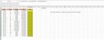
i am using the formula as shown in the pic, However this takes the account of both "Urgent" & "Non Urgent" and also i am not able to think how bring the date criteria in it.

I hope you guys understood. My english is bad its not my first language

thanks for the help in advance

 

[Eric W]

Do you mean like this?

Book1 (version 1).xlsb
	A	B	C	D	E	F	G	H
1								12-04-2020
2
3	Item	Price	Category	Date	Rank
4	CTR_01	3.5	Urgent	04-04-2020	6
5	CTR_02	3.2	Not Urgent	05-04-2020
6	CTR_03	3.44	Not Urgent	06-04-2020
7	CTR_04	3	Urgent	06-04-2020	2
8	CTR_05	2.1	Urgent	08-04-2020	1
9	CTR_06	3.4	Urgent	09-04-2020	5
10	CTR_07	3.2	Urgent	06-04-2020	4
11	CTR_08	3.44	Urgent	11-05-2020
12	CTR_09	3	Not Urgent	12-04-2020
13	CTR_10	2.1	Not Urgent	06-04-2020
14	CTR_11	3.4	Not Urgent	14-05-2020
15	CTR_12	3.2	Not Urgent	15-04-2020
16	CTR_13	3.44	Not Urgent	16-04-2020
17	CTR_14	3	Not Urgent	17-04-2020
18	CTR_15	2.1	Not Urgent	18-04-2020
19	CTR_16	3.4	Not Urgent	19-04-2020
20	CTR_17	3.2	Urgent	20-04-2020
21	CTR_18	3.44	Urgent	21-04-2020
22	CTR_19	3	Urgent	06-04-2020	2
23	CTR_20	2.1	Urgent	23-04-2020
Sheet16

Cell Formulas
Range	Formula
E4:E23	E4	=IF(AND(C4="Urgent",D4<=$H$1),SUMPRODUCT(--($B$4:$B$23<B4),--($C$4:$C$23="Urgent"),--($D$4:$D$23<=$H$1))+1,"")

 

[andrei461]

yeah eric something like this but the ranking is needed to be in series. like as in your case 3 is missing. i have found a solution though

=IF((C5="Urgent")*(D5>=H$2),MAX(1,SUM(FREQUENCY(IF((C$4:C$23="Urgent")*(D$4:D$23>$H$2)*(B$4:B$23>B5),B$4:B$23),B5))),"")

That formula solved my issue.

Thanks for your response