Refer to cells in formula using column headers

[suremac]

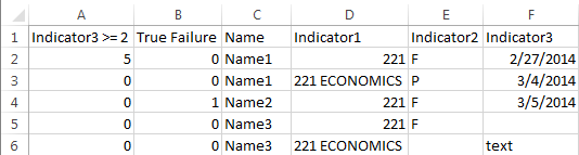
The problem is that in other versions of Sheet1, a sample of the worksheet data is provided in the image below, the data in columns C through F may be in different columns (e.g the data in column A in version 1 of Sheet1 may be in column X in version 2 of Sheet1). I'm trying to make the macro more flexible by having the formulas in the macro somehow refer to the relevant cell by using the column name (i.e. the names in row 1), instead of using only R1C1 notation.
Here is my code:

Sub Formulas()
Dim mycell As Range
With Sheets("Sheet1")
.Range("A1").EntireColumn.Insert
.Range("A1").EntireColumn.Insert
.Cells(1, 1) = "Indicator3 >= 2"
.Cells(1, 2) = "True Failure"
lr = Cells(Rows.Count, 3).End(xlUp).Row
.Range(.Cells(2, 1), .Cells(lr, 1)).FormulaR1C1 = "=IF(AND(RC[4]=""F"",(AND(ISNUMBER(SEARCH(""ECONOMICS"",R[1]C[3])),R[1]C[4]=""P"")),(ISNUMBER(R[1]C[5]))),R[1]C[5]-RC[5],0)"
.Range(.Cells(2, 2), .Cells(lr, 2)).FormulaR1C1 = "=IF(AND(RC[3]=""F"",NOT(AND(ISNUMBER(SEARCH(""ECONOMICS"",R[1]C[2])),R[1]C[3]=""P"")),(ISNUMBER(RC[4]))),1,0)"
End With
End Sub

Any help is much appreciated.
Regards,

 

[Jerry Sullivan]

Hi suremac,

You could use Application.Match to get the column number associated with each header, then use those values in your formulas.

This example uses Absolute references for the columns instead of Relative to make the notation simpler. If you need relative you can add the brackets and subtract 1 from each Column number.

Sub Formulas()
 Dim lColInd1 As Long, lColInd2 As Long, lColInd3 As Long, lr As Long

 With Sheets("Sheet1")
   .Range("A1:B1").EntireColumn.Insert
   .Cells(1, 1) = "Indicator3 >= 2"
   .Cells(1, 2) = "True Failure"
   lr = .Cells(Rows.Count, 3).End(xlUp).Row

   lColInd1 = Application.Match("Indicator1", .Rows(1), 0)
   lColInd2 = Application.Match("Indicator2", .Rows(1), 0)
   lColInd3 = Application.Match("Indicator3", .Rows(1), 0)
   
   .Range(.Cells(2, 1), .Cells(lr, 1)).FormulaR1C1 = _
      "=IF(AND(RC" & lColInd2 & "=""F"",(AND(ISNUMBER(SEARCH(""ECONOMICS""," & _
      "R[1]C" & lColInd1 & ")),R[1]C" & lColInd2 & "=""P"")),(ISNUMBER(R[1]C" & _
      lColInd3 & "))),R[1]C" & lColInd2 & "-RC" & lColInd3 & ",0)"

 End With
 
End Sub

 

[suremac]

Thank you very much! This did the trick.