Referencing cells on another sheet base on a specific text in a cell

[RSDB]

I have a spreadsheet where there are multiple data across columns in rows. On my second sheet I would like to view only 1 row's data vertically in column A. Im hoping that it can be achieved by typing a specific text in column A1 from sheet 1 with the data, and that will cause all the cells from row 1 to appear in a vertical form in Column A on sheet 2. Is this possible? and how will I go about achieving this?

 

[Joe4]

I think this would be a lot easier for us to understand if you showed us a small example of your data on Sheet1, and what you want to see on Sheet2.

MrExcel has a tool called “XL2BB” that lets you post samples of your data that will allow us to copy/paste it to our Excel spreadsheets, so we can work with the same copy of data that you are. Instructions on using this tool can be found here: XL2BB Add-in

Note that there is also a "Test Here” forum on this board. This is a place where you can test using this tool (or any other posting techniques that you want to test) before trying to use those tools in your actual posts.

 

[RSDB]

I think this would be a lot easier for us to understand if you showed us a small example of your data on Sheet1, and what you want to see on Sheet2.

MrExcel has a tool called “XL2BB” that lets you post samples of your data that will allow us to copy/paste it to our Excel spreadsheets, so we can work with the same copy of data that you are. Instructions on using this tool can be found here: XL2BB Add-in

Note that there is also a "Test Here” forum on this board. This is a place where you can test using this tool (or any other posting techniques that you want to test) before trying to use those tools in your actual posts.

Thank you, ill do just that and post a sample in XL2BB.

 

[RSDB]

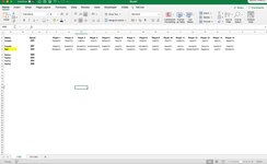
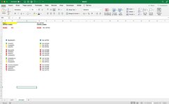
Im working on a Mac and struggling to add the Add-in. Not sure if its because its a Mac or another reason. I have taken a screenshot of the two sheets, "list" and "round".

On the "list" sheet if I type "Open" in Column A, I would like the whole row's data to be linked to cells on "Round" sheet. The information on the left in "Round" sheet is how I would like it to look and the information on the right is just to show which cells it referenced to on "List" sheet.

Hope this gives you enough information to try and help. Thank you very much in advance.

 

[Joe4]

I think you need to explain why on your "Round" sheet, the names are sorted in a different order, some rows are skipped (there are blanks in the middle of the list), and how those color coded icons are determined. It is not evident to me from what you have posted.

 

[RSDB]

There will be 15 players in a round but they split into 2 teams of 7 and player 1 being the "leader". Each position have a role in the game, hence you will see the same color combination top half of the list and bottom half of the list.

On the "List" sheet we need to see all the same positions in the columns as its listed currently for keeping track, the "Round" sheet is just for us to be able to post it to the players of the next round.

Is it possible to do something like this on excel? We have been doing it by "=" referencing the cell but need to do that for every row on "List" sheet.

 

[Joe4]

OK, I think I may see where you are going with this.
The tricky thing is that there appears to be no pattern to the columns it pulls from - they seem to jump around.
So, on the ROUND sheet, let's say that we pick some unused column (column F, in this example though you can use any column), and put the column letters that each row should pull from, like this:

Then, assuming that you also put the "Round" you want to pull from in row 4 (like in your example), then for a round in cell B4, place this formula in cell B12 and copy the formula down to cell B30, and it should return exactly what you show in your example:

=IF($F12="","",INDIRECT("List!" & $F12 & MATCH(B$4,List!$C:$C,0)))

If you wanted to add additional rounds on the same sheet, so let's say you enter a new round in cell C4. Then you could simply copy the formulas from B12:B30 to C12:C30, and it would still work.

 

[RSDB]

OK, I think I may see where you are going with this.
The tricky thing is that there appears to be no pattern to the columns it pulls from - they seem to jump around.
So, on the ROUND sheet, let's say that we pick some unused column (column F, in this example though you can use any column), and put the column letters that each row should pull from, like this:
View attachment 59428

Then, assuming that you also put the "Round" you want to pull from in row 4 (like in your example), then for a round in cell B4, place this formula in cell B12 and copy the formula down to cell B30, and it should return exactly what you show in your example:

=IF($F12="","",INDIRECT("List!" & $F12 & MATCH(B$4,List!$C:$C,0)))

If you wanted to add additional rounds on the same sheet, so let's say you enter a new round in cell C4. Then you could simply copy the formulas from B12:B30 to C12:C30, and it would still work.

Thank you thank you. amazing, it works and im thrilled. Thank you for your time to help me with this.

 

[Joe4]

You are welcome. Glad I was able to help!