Remove prefix letter in a Cell with VBA

[Pungie]

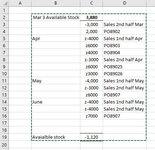
I have a simple spread sheet to run my purchase projections and in each column I have a formula. I use a simple method of adding a "Prefix" letter in front of the number in the cell to remove that cell from the calculation and then remove the "prefix" letter to get the number in cell to be included in the calculation again.

I found a VBA code to

Sub JPegMe()
Dim myCell As Range
For Each myCell In Selection
If Not IsEmpty(myCell) Then _
myCell = "z" & myCell
Next myCell
End Sub

Is there a VBA code I can use to remove the prefix?

 

[Rick Rothstein]

The best I can tell, diddi's code requires you to select the same amount of cells as my code does (namely, a range of cell that included the cells you wanted to process)... it does not look like his code would work if you only selected one cell.

 

[Pungie]

The best I can tell, diddi's code requires you to select the same amount of cells as my code does (namely, a range of cell that included the cells you wanted to process)... it does not look like his code would work if you only selected one cell.

Both your code and his both work to select 1 cell in my test spread sheet, but only his works to remove "z" from my live spread sheet (... along with the 5 in front of a cell with 5500 if I select the wrong cell . I can see it causing some real problems if I click the wrong cell and don't realize it.)
I will probably try to recreate my live spread sheet and see if your code works there. I'm sure it is a remnant of an old VB code or something else since this sheet is going on 15 years old.

 

[Rick Rothstein]

Just to repeat... select a range that includes the cells you want to process (that range can be larger if you want but for efficiency sake, you should not make it gigantic), then run my macro.... only leading Z's will be deleted, nothing else.

 

[Pungie]

Just to repeat... select a range that includes the cells you want to process (that range can be larger if you want but for efficiency sake, you should not make it gigantic), then run my macro.... only leading Z's will be deleted, nothing else.

Your code worked without any problem after I recreated my sheet and copied over the data. It was my spread sheet.
Thanks for all the help!

 

[Rick Rothstein]

Great! I am glad that you now have a working solution.

 

[diddi]

we can do a quick modify of DeleteZ to allow it to work better for you if you want

 

[Pungie]

we can do a quick modify of DeleteZ to allow it to work better for you if you want

Hi Diddi
Rick's solution works but I'm still trying to learn VBA so if it does not take too long I would love to see your solution. To be honest Rick's code was too advance for me to understand and try to manipulate in the future, but it works. ??

 

[Rick Rothstein]

Hi Diddi
Rick's solution works but I'm still trying to learn VBA so if it does not take too long I would love to see your solution. To be honest Rick's code was too advance for me to understand and try to manipulate in the future, but it works. ??

Let me see if I can explain what my formula is doing. First off, the Evaluate function simply processes Excel formulas within the VBA environment, but before I can go on, we need to understand a little about Excel formulas. If you give a formula a range of values to deal with, Excel will perform whatever calculation applies to the range one cell at a time and return an array of values. Now you cannot always see that this is the case because formulas return single values to cells, but an array of values is still calculated behind the scenes. Here is an easy demonstration of this. Put a 1 in cell A1, a 2 in cell A2 and a 3 in cell A3. Next put this formula in cell B1...

=5*A1:A3

What is returned by the formula is 5, but the formula actually calculated 5 times each value in the three cells of A1:A3. You can see this by selecting cell B1 and then selecting everything except for the equal sign in the Formula Bar after which you should press the F9 Key. What you will see is this...

{5;10;15}

That is the array of values that Excel calculated for the formula, but it did not know how to show you all three values, so it showed you just the first value. Press the ESC Key to remove the displayed array and return the formula to the Formula Bar. Now select cells B1:B3, then click into the end of the formula in the Formula Bar and press CTRL+SHIFT+ENTER (that keystroke tells the formula to return its array values to the selected array of cells)... voila, the three values of the array you saw when you pressed the F9 Key are now displayed individually in the (array of) cells you had selected.

Okay, with that backdrop, let's return to my code. As I said earlier, the Evaluate function simply processes Excel formulas within the VBA environment. Since the Selection in the With statement is a range of vertical cells, Evaluate will calculate an array of values, one value for each of those cells in Selection. Those calculated values will be placed right back into the cells that the original values came from in a manner similar to what I showed you for the selection B1:B3 after pressing the CTRL+SHIFT+ENTER keystroke.

Now let's look at the formula itself as I assume those @ signs are confusing you somewhat. They are simply place-holders for the Selection's address. Instead of having to concatenate .Address into the formula three times, I put an @ symbol where the address would go and then used VBA's Replace function to put the actual Selection address directly into the formula at each position with the place-holder @ symbol was located.

I hope the above helps you in understanding how my code works.

 

[diddi]

Rick is the guru. he answers my questions when i am stuck
if you still want my solution i can take a look

 

[Pungie]

Let me see if I can explain what my formula is doing. First off, the Evaluate function simply processes Excel formulas within the VBA environment, but before I can go on, we need to understand a little about Excel formulas. If you give a formula a range of values to deal with, Excel will perform whatever calculation applies to the range one cell at a time and return an array of values. Now you cannot always see that this is the case because formulas return single values to cells, but an array of values is still calculated behind the scenes. Here is an easy demonstration of this. Put a 1 in cell A1, a 2 in cell A2 and a 3 in cell A3. Next put this formula in cell B1...

=5*A1:A3

What is returned by the formula is 5, but the formula actually calculated 5 times each value in the three cells of A1:A3. You can see this by selecting cell B1 and then selecting everything except for the equal sign in the Formula Bar after which you should press the F9 Key. What you will see is this...

{5;10;15}

That is the array of values that Excel calculated for the formula, but it did not know how to show you all three values, so it showed you just the first value. Press the ESC Key to remove the displayed array and return the formula to the Formula Bar. Now select cells B1:B3, then click into the end of the formula in the Formula Bar and press CTRL+SHIFT+ENTER (that keystroke tells the formula to return its array values to the selected array of cells)... voila, the three values of the array you saw when you pressed the F9 Key are now displayed individually in the (array of) cells you had selected.

Okay, with that backdrop, let's return to my code. As I said earlier, the Evaluate function simply processes Excel formulas within the VBA environment. Since the Selection in the With statement is a range of vertical cells, Evaluate will calculate an array of values, one value for each of those cells in Selection. Those calculated values will be placed right back into the cells that the original values came from in a manner similar to what I showed you for the selection B1:B3 after pressing the CTRL+SHIFT+ENTER keystroke.

Now let's look at the formula itself as I assume those @ signs are confusing you somewhat. They are simply place-holders for the Selection's address. Instead of having to concatenate .Address into the formula three times, I put an @ symbol where the address would go and then used VBA's Replace function to put the actual Selection address directly into the formula at each position with the place-holder @ symbol was located.

I hope the above helps you in understanding how my code works.

Hi Rick

Wow. Thanks for the explanation
I will play around with the code a bit and try to see if I can understand it better.

You and Diddi are so awesome.