Remove text from string between parenthesis leaving only numbers

[zipotontic]

Hello!
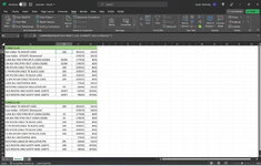
I have an inventory list with products of various units of measure (box, each, spool, etc). If it is more than 1, the total number of units is included in parenthesis at the end of the item name. So, for example, if it is a spool of 100 feet, it will show (100FT) or, if it is a box of 50, it will show (50/bx), etc.

What I am trying to achieve is a column that lists only the numeric values found between the parenthesis.

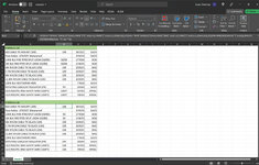
So far I have written two different formulas that extract the string between the parenthesis. However, there are issues with each. Formula 1 extracts the entire string in between the parenthesis, I cannot figure out how to modify/add to this formula so that it will remove the text and leave only the number. Formula 2 is long and clunky but it does the trick more or less. The issue is it creates a lot of work for me because I have to make sure I scan an entire list of thousands of products to be sure I have included all units of measure (so far I have only found box, spool, each). Also, occasionally there will be an item with some other random bit of information in parenthesis not related to the unit of measure and my formula will end up displaying that.

Formula #1:
=IFERROR(MID(LEFT(A2,FIND(")",A2)-1),FIND("(",A2)+1,LEN(A2)),"")

Formula #2:
IF(D16="SPOOL",MID(LEFT(A16,FIND("FT)",A16)-1),FIND("(",A16)+1,LEN(A16)),IF(D16="BOX",MID(LEFT(A16,FIND("/BX)",A16)-1),FIND("(",A16)+1,LEN(A16)),IF((ISNUMBER(SEARCH(")",A16))),RIGHT(TEXTBEFORE(A16, ")"),3),"")))

Thanks so much for the help!

 

[Micron]

Should be fairly straight forward if you're willing to drag a vba function call down this column. If not, hang on for a formula solution, but formulas are not my thing. I can see a code solution that would find the point where "(" begins and ")" ends and captures what's in between. If no leading parenthesis in the cell then nothing is returned by the function.

 

[zipotontic]

Should be fairly straight forward if you're willing to drag a vba function call down this column. If not, hang on for a formula solution, but formulas are not my thing. I can see a code solution that would find the point where "(" begins and ")" ends and captures what's in between. If no leading parenthesis in the cell then nothing is returned by the function.

Thank you so much for the response. I have nothing against VBA except that I really have zero idea how to use it. So, unless you feel like giving me a detailed instructional and a line by line function, I’m not sure I’ll be able to pull it off.

 

[Micron]

I can write that but not tonight. Too late here.
You'd drag the formula down column B (?) based on your pic, starting at B2. It would pass the value of A2 to the function, which would work as I described. If you had "( " or ")" in a header row like A15 in your pic, then that might be an issue. Otherwise should be OK. The formula is nothing more than a simple function call.

 

[johnnyL]

Try this:

Book1
	A	B	C	D	E
1	FORMULA #johnnyL
2	#10 CABLE TIE MOUNT (100)	100	381321	EACH
3	Fuse Holder ATO/ATC Waterproof		374374	EACH
4	1/4IN BLK FIRE RTRD SPLIT LOOM (50/BX)	50	177658	BOX
5	1IN BLK FIRE RTRD SPLIT LOOM (50/BX)	50	174670	BOX
6	4IN NYLON CABLE TIE BLACK (100)	100	203023	BAG
7	5.7IN NYLON CABLE TIE BLACK (100)	100	203027	BAG
8	8IN NYLON CABLE TIE BLACK (100)	100	203031	BAG
9	11.8IN NYLON CABLE TIE BLACK (100)	100	203035	BAG
10	1/8IN BLK HEATSHRINK 48IN		77818	EACH
11	ROTATING CABLECAP INSULATOR (PR)		20304	EACH
12	14/2 RED/YEL RND SAFETY WIRE (100FT)	100	92703	SPOOL
13	12/2 RED/YEL RND SAFETY WIRE (100FT)	100	78924	SPOOL
14
Sheet1

Cell Formulas
Range	Formula
B2:B13	B2	=TEXTJOIN("",TRUE,IFERROR((MID( TEXTBEFORE(TEXTAFTER(A2, "("), ")"),ROW(INDIRECT("1:"&LEN( TEXTBEFORE(TEXTAFTER(A2, "("), ")") ))),1)*1),""))

 

[Peter_SSs]

Welcome to the MrExcel board!

I suggest that you update your Account details (click your user name at the top right of the forum) so helpers always know what Excel version(s) & platform(s) you are using as the best solution often varies by version. (Don’t forget to scroll down & ‘Save’)

I also suggest that you investigate XL2BB for providing sample data to make it easier for helpers.

thousands of products

Not sure how many thousands but you may need to be a little wary of using the suggested formula from post #5 since INDIRECT is a volatile function and may slow your sheet performance. However, @johnnyL couldn't that volatile structure be replace with a SEQUENCE function since it seems the OP has a version with that available?

Another possible negative to the formula would be if data like I have in row 12 below is possible as the formula would not pick up that number.

I have nothing against VBA except that I really have zero idea how to use it. So, unless you feel like giving me a detailed instructional

I do have a vba suggestion. I have assumed that the data is in column A and column B is available for the results.
Test with a copy of your workbook.

To implement ..
1. With your workbook active press Alt+F11 to bring up the vba window.
2. In the Visual Basic window use the menu to Insert|Module
3. Copy (you can use the icon at the top-right of the forum code window) and Paste the code below into the main right hand pane that opens at step 2.
4. Close the Visual Basic window.
5. Press Alt+F8 to bring up the Macro dialog
6. Select the GetNumbers macro & click ‘Run’
7. Your workbook will need to be saved as a macro-enabled workbook (*.xlsm)

Sub GetNumbers()
  Dim RX As Object
  Dim a As Variant, b As Variant
  Dim i As Long
 
  Set RX = CreateObject("VBScript.RegExp")
  RX.Pattern = "(\([^\d\)]*)(\d+)"
  With Range("A2", Range("A" & Rows.Count).End(xlUp))
    a = .Value
    ReDim b(1 To UBound(a), 1 To 1)
    For i = 1 To UBound(a)
      If RX.test(a(i, 1)) Then b(i, 1) = RX.Execute(a(i, 1))(0).SubMatches(1)
    Next i
    .Offset(, 1).Value = b
  End With
End Sub

My sample data (thanks to @johnnyL for the XL2BB sample data) & vba results:

zipotontic.xlsm
	A	B
1
2	#10 CABLE TIE MOUNT (100)	100
3	Fuse Holder ATO/ATC Waterproof
4	1/4IN BLK FIRE RTRD SPLIT LOOM (50/BX)	50
5	1IN BLK FIRE RTRD SPLIT LOOM (50/BX)	50
6	4IN NYLON CABLE TIE BLACK (100)	100
7	5.7IN NYLON CABLE TIE BLACK (100)	100
8	8IN NYLON CABLE TIE BLACK (100)	100
9	11.8IN NYLON CABLE TIE BLACK (100)	100
10	1/8IN BLK HEATSHRINK 48IN
11	ROTATING CABLECAP INSULATOR (PR)
12	ROTATING CABLECAP INSULATOR (PR) (EACH 50)	50
13	14/2 RED/YEL RND SAFETY WIRE (100FT)	100
14	12/2 RED/YEL RND SAFETY WIRE (100FT)	100
Sheet1

 

[johnnyL]

Not sure how many thousands but you may need to be a little wary of using the suggested formula from post #5 since INDIRECT is a volatile function and may slow your sheet performance. However, @johnnyL couldn't that volatile structure be replace with a SEQUENCE function since it seems the OP has a version with that available?

Another possible negative to the formula would be if data like I have in row 12 below is possible as the formula would not pick up that number.

You are exactly right.

I stink at formulas so I just put together something that worked for the data provided. I totally missed the 'thousands' reference in the OP.

 

[Peter_SSs]

If any number to be extracted is in a set of parentheses at the end of the data like all the samples, then this might be a formula approach.

zipotontic.xlsm
	A	B
1
2	#10 CABLE TIE MOUNT (100)	100
3	Fuse Holder ATO/ATC Waterproof
4	1/4IN BLK FIRE RTRD SPLIT LOOM (50/BX)	50
5	1IN BLK FIRE RTRD SPLIT LOOM (50/BX)	50
6	4IN NYLON CABLE TIE BLACK (100)	100
7	5.7IN NYLON CABLE TIE BLACK (100)	100
8	8IN NYLON CABLE TIE BLACK (100)	100
9	11.8IN NYLON CABLE TIE BLACK (100)	100
10	1/8IN BLK HEATSHRINK 48IN
11	ROTATING CABLECAP INSULATOR (PR)
12	ROTATING CABLECAP INSULATOR (PR) (EACH 50)	50
13	14/2 RED/YEL RND SAFETY WIRE (100FT)	100
14	12/2 RED/YEL RND SAFETY WIRE (100FT)	100
Sheet2

Cell Formulas
Range	Formula
B2:B14	B2	=LET(t,TEXTAFTER(A2,"(",-1),IFERROR(CONCAT(IFERROR(MID(t,SEQUENCE(LEN(t)),1)+0,""))+0,""))

 

[johnnyL]

Since we are dealing with hypotheticals, how would
ROTATING CABLECAP INSULATOR (EACH 50) (PR)
be handled?

 

[Peter_SSs]

Since we are dealing with hypotheticals, how would
ROTATING CABLECAP INSULATOR (EACH 50) (PR)
be handled?

With the macro of course.


.. otherwise possibly this I guess?

zipotontic.xlsm
	A				E
1
2	#10 CABLE TIE MOUNT (100)				100
3	Fuse Holder ATO/ATC Waterproof
9	11.8IN NYLON CABLE TIE BLACK (100)				100
10	1/8IN BLK HEATSHRINK 48IN
11	ROTATING CABLECAP INSULATOR (PR)
12	ROTATING CABLECAP INSULATOR (PR) (EACH 50)				50
14	12/2 RED/YEL RND SAFETY WIRE (100FT)				100
15
16	ROTATING CABLECAP INSULATOR (EACH 50) (PR)				50
17	(ROTATING) (CABLECAP) INSULATOR 45 (EACH 50) (PR)				50
Sheet2

Cell Formulas
Range	Formula
E2:E3,E9:E12,E14:E17	E2	=LET(ch,MID(A2&"|",SEQUENCE(LEN(A2)+1),1),IFNA(TEXTBEFORE(TEXTAFTER(SUBSTITUTE(CONCAT(IF(ch="(",ch,IF(ch=")",ch,IFERROR(ch+0,"")))),"()",""),"("),")")+0,""))