Removing invisible characters from VBA array and dynamic formula

[Spencer500]

Hi,

I am building a VBA macro that will run VLOOKUP on user input with the following functionality:

1. Takes in user typed or pasted data from sheet "Main"
2. Ports the data from sheet "Main" to an array.
3. Array processing: Common invisible characters are removed, data is trimmed, data is casted to text to ensure the values to look up and the look-up data set are the same data type to ensure VLOOKUP will work.
4. The array then moves the data to sheet "BlankArray", where a VBA-based dynamic VLOOKUP is run on the data.

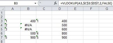
The problem is that invisible characters are somehow being created by this process, which is causing the VLOOKUP to return 500 in cell B6 from cell D4 because a match between A6 and C4 was identified by VLOOKUP. But the respective cells from sheet "Main" from which the data originated are blank.

When I select cell A6, then hit Delete, the invisible character is then deleted, which then causes VLOOKUP to return #NA in cell B6, which is what should happen if the invisible character were not in cell A6.

Invisible characters are also in cells C4 and C5. If I do not delete cell A6, and if I, instead, select C4, then hit delete, VLOOKUP returns 600 in cell B6 from D5 due to the next invisible character match between C5 and A6.

How can I modify this process to remove the invisible characters from appearing in the cells that should be blank? Also, are these invisible characters also appended to the cells that have data? If so, then how can I ensure the invisible characters are not appended to the cells with data? Do you have any other suggestions for improvements?

Please find attached workbook screenshot.

VBA Code:

Public InitialArray As Variant

Sub Match()

Sheets("Main").Select

Dim i As Long
Dim MaxFinalRow As Long


Y1 = 1
Y2 = 1
i = 1

Dim FinalRowValue As Long
Dim FinalRowKey As Long

FinalRowValue = Cells(Rows.Count, 1).End(xlUp).Row

FinalRowKey = Cells(Rows.Count, 3).End(xlUp).Row

FinalRowValueToReturn = Cells(Rows.Count, 4).End(xlUp).Row


If FinalRowValue > FinalRowKey Then
    MaxFinalRow = FinalRowValue
Else
    MaxFinalRow = FinalRowKey
End If


InitialArray = Range(Cells(3, 1), Cells(MaxFinalRow, 4))

Sheets("BlankArray").Select

Range("A1:F13").Select
Selection.ClearContents

    For i = 1 To (FinalRowValue - 2)
        InitialArray(i, 1) = Replace(InitialArray(i, 1), Chr(160), vbNullString)
        InitialArray(i, 1) = Replace(InitialArray(i, 1), Chr(10), vbNullString)
        InitialArray(i, 1) = Replace(InitialArray(i, 1), Chr(13), vbNullString)
        InitialArray(i, 1) = Replace(InitialArray(i, 1), Chr(26), vbNullString)
        InitialArray(i, 1) = Replace(InitialArray(i, 1), Chr(3), vbNullString)
        InitialArray(i, 1) = Replace(InitialArray(i, 1), Chr(28), vbNullString)
    Next i
   
    For i = 1 To (FinalRowKey - 2)
        InitialArray(i, 3) = Replace(InitialArray(i, 3), Chr(160), vbNullString)
        InitialArray(i, 3) = Replace(InitialArray(i, 3), Chr(10), vbNullString)
        InitialArray(i, 3) = Replace(InitialArray(i, 3), Chr(13), vbNullString)
        InitialArray(i, 3) = Replace(InitialArray(i, 3), Chr(26), vbNullString)
        InitialArray(i, 3) = Replace(InitialArray(i, 3), Chr(3), vbNullString)
        InitialArray(i, 3) = Replace(InitialArray(i, 3), Chr(28), vbNullString)
    Next i

    For i = 1 To (FinalRowValue - 2)
        InitialArray(i, 1) = Trim(InitialArray(i, 1))
    Next i
   
    For i = 1 To (FinalRowKey - 2)
        InitialArray(i, 3) = Trim(InitialArray(i, 3))
    Next i


For i = 1 To (FinalRowValue - 2)
    InitialArray(i, 1) = CStr(InitialArray(i, 1))
Next i


For i = 1 To (FinalRowKey - 2)
    InitialArray(i, 3) = CStr(InitialArray(i, 3))
Next i

Range(Cells(3, 1), Cells(MaxFinalRow, 4)) = InitialArray


    Range("B3").Formula = "=VLOOKUP(RC[-1],R3C3:R" & FinalRowKey & "C4,2,FALSE)"
    Range("B3").Select
    Selection.AutoFill Destination:=Range(Cells(3, 2), Cells(FinalRowValue, 2)), Type:=xlFillDefault

End Sub

Thanks.

 

[Spencer500]

Hi @Alex Blakenburg ,

Thank you for your time and expertise. From a results standpoint, your solution fixed the issue. But I am still interested in learning what caused this issue.

To reiterate from my initial post, cells A6 and C4 were visibly blank, and deleting the contents of cell A6 caused B6 to return #NA instead of 500, which appeared to indicate that there was an invisible character in cell A6 that caused it to match with the same invisible character in cell C4 to return 500. But the formulas provided by rlv01 appeared to indicate that there were no invisible characters in cell A6.

My ideal objective for this post was to identify a change to the array-based data cleansing process to prevent the apparent invisible characters from appearing in the results instead of removing the apparent invisible characters from the results. However, thus far that may not be practical because your suggested VBA code modifications still returned the apparent invisible characters that caused VLOOKUP to not function as expected because VLOOKUP with the "FALSE" exact match parameter that I used does not match blank values. It is my understanding that when using the "FALSE" exact match parameter VLOOKUP returns #NA if a match is not found for the value that is looked up or if the value that is looked up is blank.

So, what do you think caused the apparent invisible characters to appear in the results? Also, why did running Text To Columns on the results cause VLOOKUP to function as expected?

--

Hi @rlv01 ,

Per your request I, when using the version of my workbook that does not include Alex's Text To Columns VBA code, I entered "a" in cell C4. This causes VLOOKUP to return 600, which is what I would expect as noted in my interpretation of this observation from my original post as follows:

"When I select cell A6, then hit Delete, the invisible character is then deleted, which then causes VLOOKUP to return #NA in cell B6, which is what should happen if the invisible character were not in cell A6.

Invisible characters are also in cells C4 and C5. If I do not delete cell A6, and if I, instead, select C4, then hit delete, VLOOKUP returns 600 in cell B6 from D5 due to the next invisible character match between C5 and A6."

Table:

Match3.xlsm
	A	B	C	D
3	1	400	1	400
4	2	#N/A	a	500
5	3	#N/A		600
6		600	4	800
7	5	900	5	900
BlankArray

Cell Formulas
Range	Formula
B3:B7	B3	=VLOOKUP(A3,$C$3:$D$7,2,FALSE)

As noted from my response to Alex, my original objective for this post was to identify a change to the array-based data cleansing process to prevent the apparent invisible characters from appearing in the results instead of removing the apparent invisible characters from the results. Your solution does work. But it does not prevent the apparent invisible characters from appearing in the results from the VBA processing, which is my objective. Your solution could work as follows:

Match3.xlsm
	A	B	C	D
3	1	400	1	400
4	2	#N/A	a	500
5	3	#N/A		600
6			4	800
7	5	900	5	900
BlankArray

Cell Formulas
Range	Formula
B3:B7	B3	=IF(LEN(A3)>0, VLOOKUP(A3,$C$3:$D$7,2,FALSE), "")

--
Hi @Peter_SSs ,

I added the VBA from your test Subroutine at the end of the original version of my Subroutine. After running the modified Subroutine, the results are as follows:

Match5.xlsm
	A	B	C	D
3	1	400	1	400
4	2	#N/A		500
5	3	#N/A		600
6		500	4	800
7	5	900	5	900
BlankArray

Cell Formulas
Range	Formula
B3:B7	B3	=VLOOKUP(A3,$C$3:$D$7,2,FALSE)

As you can see 500 is still returned by B6, which does not match the results you provided after your comment, "Having done that my sheet now looks like this. Note changes to A10 and B6.".

Then after I delete the contents of cell A6 the results are as follows:

Match5.xlsm
	A	B	C	D
3	1	400	1	400
4	2	#N/A		500
5	3	#N/A		600
6		#N/A	4	800
7	5	900	5	900
BlankArray

Cell Formulas
Range	Formula
B3:B7	B3	=VLOOKUP(A3,$C$3:$D$7,2,FALSE)

As you can see #NA is now returned in B6 as expected because the apparent invisible character that caused A6 to match with C4 was deleted from A6.

In response to your comment:

"I suspect that cells A6, C4 & C5 originally contained formulas that returned null strings ""
Subsequently most likely a copy/paste values has occurred. This still leaves those cells with a zero length string."

Cells A6, C4 & C5 did not originally contain formulas. The values from columns A, C, and D in the final results sheet originally came from another sheet and were not formulas on that sheet. But these values were pasted into that sheet. As noted from the original VBA code that I submitted in my first post in this thread, the objective of my macro is to perform array-based processing from user inputted data from one sheet then run a VBA-based dynamic VLOOKUP on that array-processed data on a different sheet. The purpose of the array-based processing is remove common invisible characters, trim the data, and cast the column containing the values that are looked up and the column containing the look-up values both as text to ensure VLOOKUP does not fail due to comparing the same values that could initially be different data types such as 1, which could be a Number or String on the sheet where the user pastes the data.

If it is possible, my objective for this post is to make an improvement to the array-based processing on the user inputted data to prevent these apparent invisible characters from appearing in the results. Do you see any issues with Alex's CleanData Subroutine that are causing these apparent invisible characters from appearing in the results? Alex's CleanData Subroutine made improvements to my original VBA code. But the CleanData Subroutine did not prevent the apparent invisible characters from appearing in the results.

--

Thanks.

 

[Alex Blakenburg]

Great feedback.
Is there anyway you could share your sheet with the invisible characters via Drop box, Google Drive or some other sharing platform ?
At this point the only zero-length strings I can get that could in principle cause the issue is a single quote ( ' )f or a formula result ie ="".
However passing it through an array and outputting the array to BlankArray converted both of these to Empty / Blank so didn't cause the issue you are experiencing.

Just to cover off all basis, if you click in Main A6, I don't suppose you can see a single quote mark (or anything else) in the formula bar do you ?
Also unlikely but if in you stop the code straight after loading IntialArray do you just see the double quotes in (2,1)
ie

The text to columns does some conversion in the background and seems to be able to clean it up.

 

[Peter_SSs]

Like Alex, to investigate further I would like to see an actual file (with original data) and including your existing vba code.

 

[Spencer500]

Hi @Alex Blakenburg ,

When I click on Main A6, I do not see a single quote mark. The formula bar is blank.

I do not use the Watch Window. Consequently, I cannot answer your question regarding the double quotes.

The improved VBA code that you provided is in Subroutine CleanData.

It seems that porting data from a worksheet range that contains blank cells to a VBA array results in the creation of an invisible character in the respective array addresses of the blank cells. If blank values can be identified in the array by reporting string lengths of 0, then we could loop through the array to identify addresses of the array that store values that contain string lengths equal to 0 and replace the contents of these addresses with vbNullString or something similar that would not result in carrying an invisible character through to the final output in the destination sheet, which in this workbook is BlankArray.

I tried this in Subroutine CleanData2. In CleanData2, notice that I added two array traversals to perform what I noted above. But this did not work.

Per your request, the file can be downloaded at this link and will only be available for seven days:

Download

Click to download the files for this transfer with TransferNow

www.transfernow.net

Please let me know if we can modify the array data transfer and cleansing process to ensure the array does not store values that will result in invisible characters carried through to the destination worksheet when the array contents is ported to the destination worksheet.

Thanks.

 

[Peter_SSs]

Per your request, the file can be downloaded at this link and will only be available for seven days:

Looking at the the Sheet 'BlankArray' the format of columns A & C is Text. Your replacements are replacing various characters with null strings and then placing them in a Text cell so they will still be null strings.

Try adding this blue line into Sub CleanData() above the line shown

Range(Cells(3, 1), Cells(MaxFinalRow, 4)).NumberFormat = "General"
Range(Cells(3, 1), Cells(MaxFinalRow, 4)) = InitialArray

 

[Spencer500]

Hi Peter,

Thanks for this suggestion. But this will not work because the value to look up (Sheet BlankArray column A) and the lookup identifier (Sheet BlankArray column C) must be text because it possible that the value to look up and the lookup identifier on the user input worksheet Main could have leading zeros. When using your modification, those leading zeros are dropped and cause an invalid match between cell A3 and C3 resulting in 11 being returned by VLOOKUP in cell B3. In this example, the A3 user input value in Sheet Main = 0001 and the C3 user input value = 0011, which are different text values and do not match.

User input on Sheet Main:

Match_Test2_1.xlsm
	A	B	C	D
3	0001		001	0011
4	0002		0002	0012
5	0003		0003	0013
6	0004		0004	0014
7	0005		0005	0015
Main

Destination sheet BlankArray:

Match_Test2_1.xlsm
	A	B	C	D
3	1	11	1	11
4	2	12	2	12
5	3	13	3	13
6	4	14	4	14
7	5	15	5	15
BlankArray

Cell Formulas
Range	Formula
B3:B7	B3	=VLOOKUP(A3,$C$3:$D$7,2,FALSE)

If I understand your point correctly, if a null string value in the array is causing the destination cell to not be a true blank, then what should be used in place of vbNullString in the following Substitute statement:

InitialArray = Application.Substitute(InitialArray, Chr(160), vbNullString)

But in the case of the specific data in the worksheet I provided in the link, no array code should be setting any of the array addresses to vbNullString in Subroutine CleanData. To reiterate my point from last post, I think the invisible character that is causing visibly blank cells to not be true blanks is created in the array when an array address is set equal to a blank worksheet cell. But since the initial user input worksheet and the destination worksheet "value to look up" (column A) and "the lookup identifier" (column C) must be text to ensure leading zeros are not dropped, do you have an alternative solution?

I want to say also, that I really appreciate your time to assist with this question. With that said, I want to reiterate that if there is no practical solution available to ensure the blanks in the destination sheet are true blanks by changing the array process, then it may be best to end this thread and consider Alex's Text To Columns solution the most practical answer.

Please let me know your thoughts.

Thanks.

 

[Peter_SSs]

Would the simplest solution be to amend the column B formula?

Range("B3").Formula = "=IF(RC[-1]="""",NA(),VLOOKUP(RC[-1],R3C3:R" & FinalRowKey & "C4,2,FALSE))"

BTW, you can enter the whole column of formulas at once rather than taking those 3 lines of code to do it.

Range("B3:B" & FinalRowValue).Formula = "=IF(RC[-1]="""",NA(),VLOOKUP(RC[-1],R3C3:R" & FinalRowKey & "C4,2,FALSE))"

 

[Spencer500]

Hi Peter,

Yes, this solution results in VLOOKUP returning expected results and is similar to the solution suggested by rlv01.

And thanks for the tip that this can be done using one line of code. Is there any performance difference between the single line dynamic formula solution vs. using Selection.AutoFill Destination?

I have an additional question.

As noted earlier, part of the array data cleansing process is removing common invisible characters and trimming the values. But I also cast "value to look up" (column A) and "the lookup identifier" (column C) to text to ensure VLOOKUP does not fail due to comparing different data types. So is it better to run the cast statement before or after the invisible character removal and trim code?

--

Invisible Character Removal and value trimming before casting:

  InitialArray = Application.Substitute(InitialArray, Chr(160), vbNullString)
    InitialArray = Application.Substitute(InitialArray, Chr(10), vbNullString)
    InitialArray = Application.Substitute(InitialArray, Chr(13), vbNullString)
    InitialArray = Application.Substitute(InitialArray, Chr(26), vbNullString)
    InitialArray = Application.Substitute(InitialArray, Chr(3), vbNullString)
    InitialArray = Application.Substitute(InitialArray, Chr(28), vbNullString)
    
    InitialArray = Application.Trim(InitialArray)


For i = 1 To (FinalRowValue - 2)
    InitialArray(i, 1) = CStr(InitialArray(i, 1))
Next i


For i = 1 To (FinalRowKey - 2)
    InitialArray(i, 3) = CStr(InitialArray(i, 3))
Next i

--

Invisible Character Removal and value trimming after casting:

For i = 1 To (FinalRowValue - 2)
    InitialArray(i, 1) = CStr(InitialArray(i, 1))
Next i


For i = 1 To (FinalRowKey - 2)
    InitialArray(i, 3) = CStr(InitialArray(i, 3))
Next i
    
    InitialArray = Application.Substitute(InitialArray, Chr(160), vbNullString)
    InitialArray = Application.Substitute(InitialArray, Chr(10), vbNullString)
    InitialArray = Application.Substitute(InitialArray, Chr(13), vbNullString)
    InitialArray = Application.Substitute(InitialArray, Chr(26), vbNullString)
    InitialArray = Application.Substitute(InitialArray, Chr(3), vbNullString)
    InitialArray = Application.Substitute(InitialArray, Chr(28), vbNullString)
    
    InitialArray = Application.Trim(InitialArray)

--

Is it ok if I "Mark as Solution" more than one post in this thread?

Thanks.

 

[Peter_SSs]

Is it ok if I "Mark as Solution" more than one post in this thread?

You can't.

In relation to your other questions you are probably best to set up some larger dummy sample data and do some tests yourself.

 

[Alex Blakenburg]

If you really want to follow your original concept through, then leave columns 1 & 3 formatted as text and replace this line:

Range(Cells(3, 1), Cells(MaxFinalRow, 4)) = InitialArray

With this:

Dim OutputArray() As Variant
ReDim OutputArray(1 To UBound(InitialArray, 1), 1 To UBound(InitialArray, 2))
Dim j As Long

For i = 1 To UBound(InitialArray, 1)
    For j = 1 To UBound(InitialArray, 2)
        If InitialArray(i, j) <> vbNullString Then
            OutputArray(i, j) = InitialArray(i, j)
        End If
    Next j
Next i

Range(Cells(3, 1), Cells(MaxFinalRow, 4)) = OutputArray

What it does is this: