Rename PivotTable name in VBA

[MPaulus]

I have a macro that creates a new pivot table and the pivot table will then always have new name so I have renamed my pivot table to my sheet name, "Pivot", and now when I try to hide a column I am getting a run time error '1004': Unable to set the orientation property of the PivotField class.

 Dim ws      As Worksheet
    Dim pts     As PivotTables
    Dim pt      As PivotTable

    Set ws = ActiveSheet
    Set pts = ActiveSheet.PivotTables
    If pts.Count < 1 Then Exit Sub
    Set pt = ws.PivotTables(1)
    pt.Name = ws.Name
    
    ActiveSheet.PivotTables("Pivot").PivotFields("Future").Orientation = xlHidden

Or would it work better to name the pivot table while I am creating it, what would that code look like?

 

[Domenic]

You'll get that error whenever . . .

1) the pivot field doesn't exists, or

2) the pivot field is already hidden

Is either one the case?

 

[MPaulus]

No, the field existed and had not been previously hidden. I have found a workaround.

 

[Domenic]

That's great, glad you were able to come up with a solution.

Cheers!

 

[MPaulus]

But now I am having trouble renaming a PivotChart in a macro. I have a capacity report to run weekly that I will recreate a new pivot table and then a new chart once the data is sorted. The attached file shows the completed pivot table and the macro is where I am at in creating the table. The macro runs up to the point where I need to rename the chart so I can set the scale on the secondary axis to match the primary axis. Here is what I have written:

Sub CreateChart_Test()
'

' RenamePivotTables Macro
    Dim ws      As Worksheet
    Dim pts     As PivotTables
    Dim pt      As PivotTable

    Set ws = ActiveSheet
    Set pts = ActiveSheet.PivotTables
    If pts.Count < 1 Then Exit Sub
    Set pt = ws.PivotTables(1)
    pt.Name = ws.Name
    
'   Create Chart
    ActiveSheet.Shapes.AddChart2(201, xlColumnClustered).Select
    ActiveChart.SetSourceData Source:=Range("Pivot!$J$11:$S$19")
    ActiveChart.FullSeriesCollection(1).ChartType = xlColumnClustered
    ActiveChart.FullSeriesCollection(1).AxisGroup = 1
    ActiveChart.FullSeriesCollection(2).ChartType = xlColumnClustered
    ActiveChart.FullSeriesCollection(2).AxisGroup = 1
    ActiveChart.FullSeriesCollection(3).ChartType = xlColumnClustered
    ActiveChart.FullSeriesCollection(3).AxisGroup = 1
    ActiveChart.FullSeriesCollection(4).ChartType = xlColumnClustered
    ActiveChart.FullSeriesCollection(4).AxisGroup = 1
    ActiveChart.FullSeriesCollection(5).ChartType = xlColumnClustered
    ActiveChart.FullSeriesCollection(5).AxisGroup = 1
    ActiveChart.FullSeriesCollection(6).ChartType = xlLine
    ActiveChart.FullSeriesCollection(6).AxisGroup = 1
    ActiveChart.FullSeriesCollection(7).ChartType = xlLine
    ActiveChart.FullSeriesCollection(7).AxisGroup = 1
    ActiveChart.FullSeriesCollection(8).ChartType = xlLine
    ActiveChart.FullSeriesCollection(8).AxisGroup = 1
    ActiveChart.FullSeriesCollection(9).ChartType = xlLine
    ActiveChart.FullSeriesCollection(9).AxisGroup = 1
    ActiveChart.FullSeriesCollection(6).ChartType = xlColumnClustered
    ActiveChart.FullSeriesCollection(7).AxisGroup = 2
    ActiveChart.FullSeriesCollection(8).AxisGroup = 2
    ActiveChart.FullSeriesCollection(9).AxisGroup = 2
    ActiveChart.FullSeriesCollection(7).ChartType = xlColumnStacked
    ActiveChart.FullSeriesCollection(8).ChartType = xlColumnStacked
    ActiveChart.FullSeriesCollection(9).ChartType = xlColumnStacked

'   RenameChart
    Dim cob     As ChartObjects
    Dim cht      As Chart

    Set ws = ActiveSheet
    Set cob = ActiveSheet.ChartObjects
    If cob.Count < 1 Then Exit Sub
    Set cht = ws.ChartObjects
    cht.Name = ws.Name

'   Set Secondary Axis to match same scale as Primary Axis
    Dim x As Long


    With ActiveSheet.ChartObjects(Pivot).Chart

        ActiveSheet.ChartObjects(Pivot).Activate
        ActiveChart.Axes(xlValue).MaximumScaleIsAuto = True
        ActiveChart.Axes(xlValue).MinimumScale = 0
        x = ActiveChart.Axes(xlValue).MaximumScale
        ActiveChart.Axes(xlValue, xlSecondary).MaximumScale = x

    End With
End Sub

Chart Trouble.xlsm
	A	B	C	D	E	F	G	H	I	J	K	L	M	N	O	P	Q	R	S	T
1
2
3
4
5
6
7
8
9
10
11										Row Labels	Sum of Total Late Hrs	Sum of 10/25/2021	Sum of 11/1/2021	Sum of 11/8/2021	Sum of 11/15/2021	Sum of 11/22/2021	Sum of 40 Hr Capacity	Sum of 50 Hr Capacity	Sum of 60 Hr Capacity
12										FORM	2266.59	950.07	677.26	592.85	393.13	200.24	550.69	137.6725	137.6725
13										LASER	956.84	488.1	487.85	248.27	291.04	109.15	213.04	53.26	53.26
14										LASER UNLOAD	1299.87	568.36	486.44	308.59	316.94	112.05	611.05	152.7625	152.7625
15										N/A	4021.92	889.37	788.57	1007.71	881.84	522.35	694.59	173.6475	173.6475
16										PAINT	165.69	87.82	52.04	82.19	22.95	19.53	234.9	58.725	58.725
17										TURRETS	853.46	277.09	227.44	138.33	123.19	88.07	213.04	53.26	53.26
18										WELD	4039.59	1071.85	1354.08	1237.79	835.97	384.56	1024.54	256.135	256.135
19										Grand Total	13603.96	4332.66	4073.68	3615.73	2865.06	1435.95	3541.85	885.4625	885.4625
20
Pivot

 

[Domenic]

First of all, Set cht = ws.ChartObjects should produce an error since you're assigning ChartObjects to a variable that has been declared as Chart. So it should be . . .

Set cht = ws.ChartObjects(1).Chart

.

Then, to rename the chart, you'll need to refer to the ChartObject, not the Chart. So it should be . . .

cht.Parent.Name = ws.Name

Note, however, your macro can be re-written as follows...

Sub CreateChart_Test()

    If ActiveSheet.PivotTables.Count < 1 Then Exit Sub
    
    Dim ws As Worksheet
    Set ws = ActiveSheet

'   Rename PivotTable
    Dim pt As PivotTable
    Set pt = ws.PivotTables(1)
    pt.Name = ws.Name

'   Create and rename Chart
    Dim shp As Shape
    Set shp = ws.Shapes.AddChart2(201, xlColumnClustered)
    shp.Name = ws.Name
    
    With shp.Chart
        .SetSourceData Source:=pt.TableRange2
        With .FullSeriesCollection(1)
            .ChartType = xlColumnClustered
            .AxisGroup = 1
        End With
        'etc
        '
        '
    End With

'   Set Secondary Axis to match same scale as Primary Axis
    With shp.Chart
        .Axes(xlValue).MaximumScaleIsAuto = True
        .Axes(xlValue).MinimumScale = 0
        .Axes(xlValue, xlSecondary).MaximumScale = .Axes(xlValue).MaximumScale
    End With
    
End Sub

Hope this helps!

 

[MPaulus]

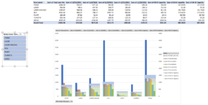
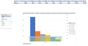
Yes, that was great! One thing just seems to lead to the next....my next step is to add a slicer based on the work centers from the right hand column. When I select one of the work centers from the slicer it keeps my secondary axis scale locked at the the summary level and doesn't adjust it to match the work center.

 

[MPaulus]

Yes, that was great! One thing just seems to lead to the next....my next step is to add a slicer based on the work centers from the right hand column. When I select one of the work centers from the slicer it keeps my secondary axis scale locked at the the summary level and doesn't adjust it to match the work center.


View attachment 49925View attachment 49926

 

[Domenic]

That's great, glad I could help.

For a new question, though, please start a new thread and ask your question there.

Cheers!