Return a calculate Arrival Date

[Codfadder]

Hi,
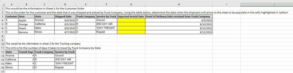
I have two separate worksheets. One worksheet has a list of Trucking Companies. Those trucking companies deliver to different States. Each of those Trucking Companies also has different types of services that they can provide. Such as Ground Service, Next Day Delivery Service, Air Service, etc. Next, I have customer shipments that were processed and picked up by those Truck Companies. Based on the Truck Service that I selected to ship the order to the customer, I need to figure out what the 'Expected Delivery Date will be for the shipment to arrive at the customer based on the State that it is being delivered to. I attached a mini - sheet as an example. I highlighted the column where I would like to have a formula that would return an 'Expected Delivery Date' for the shipment based on the date that I shipped the shipment and using the Truck Company's number of days that it will take to reach it's destination.

 

[sprigelz]

Try this in G4 and copy down;

=D4+INDEX(B$13:B$16,MATCH(F4,D$13:D$16,0))

This only matches the type "Service by Truck" columns. If you have different companies that also have varying transit days, we would also need to include the Company AND Transit by Service.

 

[Codfadder]

We are close, but I should have provided you with more details. I am adding another image with side by side tables with some information wedge between them explaining in further details of what I'm trying to achieve. Hope this is more helpful.

 

[sprigelz]

This gets you closer, and maybe someone else can jump in here to assist with the final piece. The problem with this formula as it is;
A) It's an array and depending on how many times it is duplicated it can drastically slow down your Excel sheet
B) It doesn't actually match how you have the data currently formatted. For example, it tries to match D2 with column P. However those do not match, so you would have to change one or the other throughout your entire dataset to match them up, or create a more complex formula to account for this. Alternatively, you could create a hidden helper column. A few different options available.

=INDEX(Q:Q,MATCH(1,(B2=N:N)*(C2=O:O)*(D2=P:P),0))+E2

For testing purposes, if you change D2 = "Ground", the formula should not result in an error.

 

[Codfadder]

Man, you are good. And I agree with you, it does labor a bit because of the array. But, I'm not too concern about that at the moment. I do want to apologies for not matching up the Service levels D & P before sending the information. That should have been realized. As you suggested, I updated the the columns to match and it return the date as expected. Although there is one more thing that I also should had added, which is a bit of an anomaly. And that is, if the Trucking Table does not have a 'State' then it should use the default values. I've added the further details in the uploaded images.

 

[sprigelz]

Apologies for the delay!

Try this with your original data structure;

=IFERROR(INDEX(Q:Q,MATCH(1,(B2=N:N)*(C2=O:O)*(D2=P:P),0))+E2,INDEX(Q:Q,MATCH(1,(C2=O:O)*(D2=P:P),0))+E2)

It looks like you might've changed the columns that the data lives in. Based on your most recent screenshot, this should work;

=IFERROR(INDEX(N:N,MATCH(1,(B2=K:K)*(C2=L:L)*(D2=M:M),0))+E2,INDEX(N:N,MATCH(1,(C2=L:L)*(D2=M:M),0))+E2)

 

[Codfadder]

Wow, beautiful piece of work!!. Cheers mate. This formula will go a long ways for me. This will get me some brownies for sure.. Can't thank you enough. Well done and have an awesome day.