Return multiple column headers based on value between two numbers

[angie2011]

I have been looking for days trying to find how to do this but not having much luck. I am not totally new to writing the complex formulas but haven't used them in a long time (and array has been totally new these last few weeks). I am trying to pull tech names to sheet1 based on the distance they are away from a site (0.01-50 miles, 51-100, 101-150 etc...
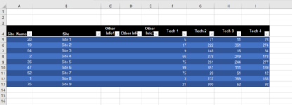
I have the table in Mileage! that shows all techs in columns (4), sites in rows (B)
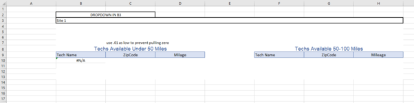
Drop down box is on sheet1 cell B3.
I have been trying to figure out the formula and this is the closest I can come up with
=(INDEX(Mileage!$F$4:$I$4,1,SMALL(IF(INDEX(Mileage!$F$5:$I$13,MATCH($B$3,Mileage!$B$5:$B$13,0),)<=50,COLUMN($A$1:$G$1)),ROW(1:1))))
which is giving me an #N/A, if I play with it enough I will end up with a #value!.
Can anyone help?
I have uploaded my sample sheet.
thank you so much for taking the time to even read and respond.

	DROPDOWN IN B3
	Site 1
		use .01 as low to prevent pulling zero
	Techs Available Under 50 Miles		Techs Available 50-100 Miles
	Tech Name	ZipCode	Milage		Tech Name	ZipCode	Mileage
	#N/A​

Site_Name	Site	Other Info1	Other Info2	Other Info3	Tech 1	Tech 2	Tech 3	Tech 4
20​	Site 1				5​	71​	11​	23​
19​	Site 2				17​	222​	361​	274​
54​	Site 3				9​	148​	16​	34​
2​	Site 4				66​	278​	249​	178​
36​	Site 5				75​	261​	244​	277​
47​	Site 6				99​	351​	111​	139​
52​	Site 7				75​	20​	61​	12​
1​	Site 8				3​	237​	389​	168​
75​	Site 9				21​	300​	62​	92​

 

[Toadstool]

Hi Angie2011,

You have 365 so I'm sure there will be a better solution along but here's my Excel 2016 approach.
NOTE: I couldn't see where the ZipCode came from so I've left that out.

Angie2011.xlsx
	A	B	C	D	E	F	G	H	I
1
2		Site Selection
3		Site 1
4
5
6
7
8		Techs Available Under 50 Miles				Techs Available 50-100 Miles
9		Tech Name	ZipCode	Mileage		Tech Name	ZipCode	Mileage
10		Tech 1		5		Tech 2		71
11		Tech 3		11
12		Tech 4		23
13
14	Site_Name	Site	Other Info1	Other Info2	Other Info3	Tech 1	Tech 2	Tech 3	Tech 4
15	20	Site 1				5	71	11	23
16	19	Site 2				17	222	361	274
17	54	Site 3				9	148	16	34
18	2	Site 4				66	278	249	178
19	36	Site 5				75	261	244	277
20	47	Site 6				99	351	111	139
21	52	Site 7				75	20	61	12
22	1	Site 8				3	237	389	168
23	75	Site 9				21	300	62	92
Sheet1

Cell Formulas
Range	Formula
D10:D12	D10	=IFERROR(INDEX($F$15:$I$23,MATCH($B$3,$B$15:$B$23,0),AGGREGATE(15,6,COLUMN($F$14:$I$14)-COLUMN($E$14)/(($F$15:$I$23<50)*($B$15:$B$23=$B$3)),ROW()-ROW($B$9))),"")
H10:H12	H10	=IFERROR(INDEX($F$15:$I$23,MATCH($B$3,$B$15:$B$23,0),AGGREGATE(15,6,COLUMN($F$14:$I$14)-COLUMN($E$14)/(($F$15:$I$23>=50)*($F$15:$I$23<=100)*($B$15:$B$23=$B$3)),ROW()-ROW($B$9))),"")
B10:B12	B10	=IFERROR(INDEX($F$14:$I$14,,AGGREGATE(15,6,COLUMN($F$14:$I$14)-COLUMN($E$14)/(($F$15:$I$23<50)*($B$15:$B$23=$B$3)),ROW()-ROW($B$9))),"")
B13	B13	=IFERROR(INDEX($F$14:$I$14,,AGGREGATE(15,6,COLUMN($F$14:$I$14)-COLUMN($E$14)/(($F$15:$I$23<=50)*($B$15:$B$23=$B$3)),ROW()-ROW($B$9))),"")
F10:F13	F10	=IFERROR(INDEX($F$14:$I$14,,AGGREGATE(15,6,COLUMN($F$14:$I$14)-COLUMN($E$14)/(($F$15:$I$23>=50)*($F$15:$I$23<=100)*($B$15:$B$23=$B$3)),ROW()-ROW($B$9))),"")

Cells with Data Validation
Cell	Allow	Criteria
B3	List	=$B$15:$B$23

 

[AhoyNC]

Maybe something like this:

Book1
	A	B	C	D	E	F	G	H	I
1	Find Site	Site 1
2		Less than 50	50-100
3		Tech 1	Tech 2
4		Tech 3
5		Tech 4
6
7
8
9	Site_Name	Site	Other Info1	Other Info2	Other Info3	Tech 1	Tech 2	Tech 3	Tech 4
10	20	Site 1				5	71	11	23
11	19	Site 2				17	222	361	274
12	54	Site 3				9	148	16	34
13	2	Site 4				66	278	249	178
14	36	Site 5				75	261	244	277
15	47	Site 6				99	351	111	139
16	52	Site 7				75	20	61	12
17	1	Site 8				3	237	389	168
18	75	Site 9				21	300	62	92
Sheet1

Cell Formulas
Range	Formula
B3:B5	B3	=TRANSPOSE(FILTER($F$9:$I$9,INDEX(F10:I18,MATCH($B$1,$B$10:$B$18,0),0)<50,"No Match"))
C3	C3	=TRANSPOSE(FILTER($F$9:$I$9,(INDEX(F10:I18,MATCH($B$1,$B$10:$B$18,0),0)>=50)*(INDEX(F10:I18,MATCH($B$1,$B$10:$B$18,0),0)<100),"No Match"))
Dynamic array formulas.

 

[angie2011]

For these formulas I get an error saying the filter function is not valid, but the first formula given above does work.
Thank you for your help. I cannot be more grateful.

 

[angie2011]

Hi Angie2011,

You have 365 so I'm sure there will be a better solution along but here's my Excel 2016 approach.
NOTE: I couldn't see where the ZipCode came from so I've left that out.

Toadstool - I cannot thank you enough for the above. I was a little confused with the aggregate function (15,6) but looked it up and was able to make the change in row B9 to move the formula to my actual sheet. This is so amazing!

 

[Toadstool]

You're welcome!
Thanks for the feedback.

You already had SMALL so I figured you'd figure AGGREGATE.

Of course if you parameterized the mileage bands it would mean less formulae

Angie2011.xlsx
	A	B	C	D	E	F	G	H	I
1
2		Site Selection
3		Site 1
4
5
6			Between miles				Between miles
7		Techs Available	0	50		Techs Available 50-100 Miles	50	100
8		Tech Name	ZipCode	Mileage		Tech Name	ZipCode	Mileage
9		Tech 1		5		Tech 2		71
10		Tech 3		11
11		Tech 4		23
12
13	Site_Name	Site	Other Info1	Other Info2	Other Info3	Tech 1	Tech 2	Tech 3	Tech 4
14	20	Site 1				5	71	11	23
15	19	Site 2				17	222	361	274
16	54	Site 3				9	148	16	34
17	2	Site 4				66	278	249	178
18	36	Site 5				75	261	244	277
19	47	Site 6				99	351	111	139
20	52	Site 7				75	20	61	12
21	1	Site 8				3	237	389	168
22	75	Site 9				21	300	62	92
V2

Cell Formulas
Range	Formula
F9:F12,B9:B12	B9	=IFERROR(INDEX($F$13:$I$13,,AGGREGATE(15,6,COLUMN($F$13:$I$13)-COLUMN($E$13)/(($F$14:$I$22>=C$7)*($F$14:$I$22<=D$7)*($B$14:$B$22=$B$3)),ROW()-ROW($B$8))),"")
H9:H12,D9:D12	D9	=IFERROR(INDEX($F$14:$I$22,MATCH($B$3,$B$14:$B$22,0),AGGREGATE(15,6,COLUMN($F$13:$I$13)-COLUMN($E$13)/(($F$14:$I$22>=C$7)*($F$14:$I$22<=D$7)*($B$14:$B$22=$B$3)),ROW()-ROW($B$8))),"")

Cells with Data Validation
Cell	Allow	Criteria
B3	List	=$B$14:$B$22