Return Multiple Result Two Dimensions

[zaki1979]

Dear Expert,

I am working in a small project. I have attached my simple data (Input & output)

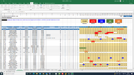
Master Data Sheet looks like as follows:

Employee ID Client Name Site Name 01/02 02/02 03/02 04/02 05/02 06/02 07/02 08/02
201101 Client A Site X P P A
201101 Client B Site Y P P P
201101 Client C Site Z P A and till the end of the Month of February 2022 (Where P represents Present & A represents Absent)

I have another Sheets (Output Sheet)/Report which will display only unique employee Id I want the result to be displayed as follows:

Employee ID 01/02 02/02 03/02 04/02 05/02 06/02 07/02 08/02 .................................28/02
201101 P P A P P P P A.
201102
201103
etc...

I know that I have to use Index/Match but unfortunately I couldn't solve the task. Is there a way to use Index/Match with Offset
any solution will be highly appreciated.

Many thanks in advance for your precious time and consideration. Looking forward to hear from you as soon as possible.





Kindly note that I am using office 2019.

 

[zaki1979]

output sheet

my project.xlsx
	A	B	C	D	E	F	G	H	I	J	K	L	M	N	O	P	Q	R	S	T	U	V	W	X	Y	Z	AA	AB	AC	AD	AE	AF
3	MATRICULE	FONCTION	01	02	03	04	05	06	07	08	09	10	11	12	13	14	15	16	17	18	19	20	21	22	23	24	25	26	27	28	TOTAL PRESENCE	TOTAL ABSENCE
4	201101	GUARDE	P	P	P	P	P	P	P	P	P	P	P	P	P	P	P	P	P	P	P	P	P	A	A	P	P	P	R	P	25	2
5	201102	GUARDE	P	P	P	P	P	P	P	P	P	P	P	P	P	P	P	P	P	P	P	P	P	P	M	M	M	M	P	P	24	0
6	201103	GUARDE	P	P	P	P	P	P	P	A	A	P	P	P	P	P	P	P	P	P	P	P	P	P	P	P	P	P	P	P	26	2
7	201104	GUARDE	0	0	0	0	0	0	0	0	0	0	0	0	0	0	0	0	0	0	0	0	0	0	0	0	0	0	0	0	0	0
8	201105	GUARDE	0	0	0	0	0	0	0	0	0	0	0	0	0	0	0	0	0	0	0	0	0	0	0	0	0	0	0	0	0	0
9	201106	GUARDE	0	0	0	0	0	0	0	0	0	0	0	0	0	0	0	0	0	0	0	0	0	0	0	0	0	0	0	0	0	0
10	201107	GUARDE	0	0	0	0	0	0	0	0	0	0	0	0	0	0	0	0	0	0	0	0	0	0	0	0	0	0	0	0	0	0
ATTENDANCE REPORT

Cell Formulas
Range	Formula
C4:AD10	C4	=INDEX('MASTER DATA'!$A$1:$AJ$11,MAX(IF('MASTER DATA'!$A$8:$A$11=$A4,IF('MASTER DATA'!$I$8:$AJ$11<>"",IF('MASTER DATA'!$I$7:$AJ$7=C$3,ROW('MASTER DATA'!$A$8:$A$11))))),MATCH(C$3,'MASTER DATA'!$A$7:$AJ$7,0))
AE4:AE10	AE4	=COUNTIF(C4:AD4,"P")
AF4:AF10	AF4	=COUNTIF(C4:AD4,"A")
Press CTRL+SHIFT+ENTER to enter array formulas.

 

[zaki1979]

Dear Sir,

Master Sheet:

my project.xlsx
	A	B	C	D	E	F	G	H	I	J	K	L	M	N	O	P	Q	R	S	T	U	V	W	X	Y	Z	AA	AB	AC	AD	AE	AF	AG	AH	AI	AJ
7	MATRICULE	NOM	ÉQUIPE	FONCTION	CLIENT	SITE	REMARQUES	UNIQUE_ID	01	02	03	04	05	06	07	08	09	10	11	12	13	14	15	16	17	18	19	20	21	22	23	24	25	26	27	28
8	201101	MIDO MIWUMBU	A	GUARDE	CLIENT 1	SITE A	RAS	201101_8	P	P	P	P	P	P	P	P	P	P	P	P	P	P	P	P	P	P
9	201102	AKANGA ALONDO	A	GUARDE	CLIENT 2	SITE B	RAS	201102_9	P	P	P	P	P	P	P	P	P	P	P	P	P	P	P	P	P	P	P	P	P	P	M	M	M	M	P	P
10	201103	INGANGE EYENGA	B	GUARDE	CLIENT 3	SITE C	RAS	201103_10	P	P	P	P	P	P	P	A	A	P	P	P	P	P	P	P	P	P	P	P	P	P	P	P	P	P	P	P
11	201101	MIDO MIWUMBU	A	GUARDE	CLIENT 4	SITE D	TRANSFERT #101	201101_11																			P	P	P	A	A	P	P	P	R	P
12	201104	TEST 1	AB	GUARDE	CLIENT 5	SITE E		201104_12																											P	P
13	201105	TEST 2	A	GUARDE	CLIENT 1	SITE A		201105_13									P											P
14	201106	TEST 3	A	GUARDE	CLIENT 7	SITE F		201106_14					P	P	P
15	201107	TEST 4	A	GUARDE	CLIENT 8	SITE G		201107_15	P	P	P	A	A	A	P	P															P					P
16	201107	TEST 4	A	GUARDE	CLIENT 2	SITE B		201107_16									R	P	P	R	A	A	A	P	A
MASTER DATA

Cell Formulas
Range	Formula
H8:H16	H8	=A8&"_"&ROW()

Cells with Conditional Formatting
Cell	Condition		Cell Format	Stop If True
I8:AJ16	Cell Value	="R"	text	NO
I8:AJ16	Cell Value	="M"	text	NO
I8:AJ16	Cell Value	="A"	text	NO
I8:AJ16	Cell Value	="P"	text	NO

Output Sheet/Report

my project.xlsx
	A	B	C	D	E	F	G	H	I	J	K	L	M	N	O	P	Q	R	S	T	U	V	W	X	Y	Z	AA	AB	AC	AD	AE	AF
3	MATRICULE	FONCTION	01	02	03	04	05	06	07	08	09	10	11	12	13	14	15	16	17	18	19	20	21	22	23	24	25	26	27	28	TOTAL PRESENCE	TOTAL ABSENCE
4	201101	GUARDE	P	P	P	P	P	P	P	P	P	P	P	P	P	P	P	P	P	P	P	P	P	A	A	P	P	P	R	P	25	2
5	201102	GUARDE	P	P	P	P	P	P	P	P	P	P	P	P	P	P	P	P	P	P	P	P	P	P	M	M	M	M	P	P	24	0
6	201103	GUARDE	P	P	P	P	P	P	P	A	A	P	P	P	P	P	P	P	P	P	P	P	P	P	P	P	P	P	P	P	26	2
7	201104	GUARDE	0	0	0	0	0	0	0	0	0	0	0	0	0	0	0	0	0	0	0	0	0	0	0	0	0	0	0	0	0	0
8	201105	GUARDE	0	0	0	0	0	0	0	0	0	0	0	0	0	0	0	0	0	0	0	0	0	0	0	0	0	0	0	0	0	0
9	201106	GUARDE	0	0	0	0	0	0	0	0	0	0	0	0	0	0	0	0	0	0	0	0	0	0	0	0	0	0	0	0	0	0
10	201107	GUARDE	0	0	0	0	0	0	0	0	0	0	0	0	0	0	0	0	0	0	0	0	0	0	0	0	0	0	0	0	0	0
ATTENDANCE REPORT

Cell Formulas
Range	Formula
C4:AD10	C4	=INDEX('MASTER DATA'!$A$1:$AJ$11,MAX(IF('MASTER DATA'!$A$8:$A$11=$A4,IF('MASTER DATA'!$I$8:$AJ$11<>"",IF('MASTER DATA'!$I$7:$AJ$7=C$3,ROW('MASTER DATA'!$A$8:$A$11))))),MATCH(C$3,'MASTER DATA'!$A$7:$AJ$7,0))
AE4:AE10	AE4	=COUNTIF(C4:AD4,"P")
AF4:AF10	AF4	=COUNTIF(C4:AD4,"A")
Press CTRL+SHIFT+ENTER to enter array formulas.

 

[DanteAmor]

You must adapt the formula, in this case change the "11" for the last row with data from the "MASTER DATA" sheet.

=INDEX('MASTER DATA'!$A$1:$AJ$11,MAX(IF('MASTER DATA'!$A$8:$A$11=$A4,IF('MASTER DATA'!$I$8:$AJ$11<>"",IF('MASTER DATA'!$I$7:$AJ$7=C$3,ROW('MASTER DATA'!$A$8:$A$11))))),MATCH(C$3,'MASTER DATA'!$A$7:$AJ$7,0))

For example:

=INDEX('MASTER DATA'!$A$1:$AJ$16,MAX(IF('MASTER DATA'!$A$8:$A$16=$A4,IF('MASTER DATA'!$I$8:$AJ$16<>"",IF('MASTER DATA'!$I$7:$AJ$7=C$3,ROW('MASTER DATA'!$A$8:$A$16))))),MATCH(C$3,'MASTER DATA'!$A$7:$AJ$7,0))

Press CTRL+SHIFT+ENTER to enter array formulas.

 

[zaki1979]

Dear sir,

Many thanks for the effort you did for me, actually it stills not working in my original data. Those ZERO's are annoying. Kindly note that check the formula again.
Please find below the report in my Original Project

PAYROLL SYSTEM.xlsm
	A	B	C	D	E	F	G	H	I	J	K	L	M	N	O	P	Q	R	S	T	U	V	W	X	Y	Z	AA	AB	AC	AD	AE	AF	AG	AH
13	MATRICULE	NOM ET POST NOM	FONCTION	EQUIPE	01	02	03	04	05	06	07	08	09	10	11	12	13	14	15	16	17	18	19	20	21	22	23	24	25	26	27	28	JOUR PRESTÉ	JOUR ABSENCE
RP03

Cell Formulas
Range	Formula
F13:AF13	F13	=E13+1

 

[DanteAmor]

I show you how it works well for me.

varios 08jun2022b.xlsm
	A	B	C	D	E	F	G	H	I	J	K	L	M	N	O	P	Q	R	S	T	U	V	W	X	Y	Z	AA	AB	AC	AD	AE	AF
1
2
3	MATRICULE	FONCTION	01	02	03	04	05	06	07	08	09	10	11	12	13	14	15	16	17	18	19	20	21	22	23	24	25	26	27	28	TOTAL PRESENCE	TOTAL ABSENCE
4	201101	GUARDE	P	P	P	P	P	P	P	P	P	P	P	P	P	P	P	P	P	P	P	P	P	A	A	P	P	P	R	P	25	2
5	201102	GUARDE	P	P	P	P	P	P	P	P	P	P	P	P	P	P	P	P	P	P	P	P	P	P	M	M	M	M	P	P	24	0
6	201103	GUARDE	P	P	P	P	P	P	P	A	A	P	P	P	P	P	P	P	P	P	P	P	P	P	P	P	P	P	P	P	26	2
7	201104	GUARDE	0	0	0	0	0	0	0	0	0	0	0	0	0	0	0	0	0	0	0	0	0	0	0	0	0	0	P	P	2	0
8	201105	GUARDE	0	0	0	0	0	0	0	0	P	0	0	0	0	0	0	0	0	0	0	P	0	0	0	0	0	0	0	0	2	0
9	201106	GUARDE	0	0	0	0	P	P	P	0	0	0	0	0	0	0	0	0	0	0	0	0	0	0	0	0	0	0	0	0	3	0
10	201107	GUARDE	P	P	P	A	A	A	P	P	R	P	P	R	A	A	A	P	A	0	0	0	0	0	P	0	0	0	0	P	10	7
Atrtendance report

Cell Formulas
Range	Formula
C4:AD10	C4	=INDEX('Master data'!$A$1:$AJ$16,MAX(IF('Master data'!$A$8:$A$16=$A4,IF('Master data'!$I$8:$AJ$16<>"",IF('Master data'!$I$7:$AJ$7=C$3,ROW('Master data'!$A$8:$A$16))))),MATCH(C$3,'Master data'!$A$7:$AJ$7,0))
AE4:AE10	AE4	=COUNTIF(C4:AD4,"P")
AF4:AF10	AF4	=COUNTIF(C4:AD4,"A")
Press CTRL+SHIFT+ENTER to enter array formulas.

 

[zaki1979]

Dear sir,

Many thanks for the effort you did for me, actually it stills not working in my original data. Those ZERO's are annoying. Kindly note that check the formula again.
Please find below the report in my Original Project

the formula isn't working correctly the output is not identical with the input. When I put the Formula in my project it is not working. I can't send you the whole data because of cell's limit to 3000 cells. In some cells it's giving #value error

waiting to hear from you.

Master Data = ATTENDANCE SHEET

New Microsoft Excel Worksheet.xlsx
	A	B	C	D	E	F	G	H	I	J	K	L	M	N	O	P	Q	R	S	T	U	V	W	X	Y	Z	AA	AB	AC	AD	AE	AF	AG	AH	AI	AJ	AK	AL	AM	AN	AO	AP	AQ	AR
1
2																																					MOIS		Feb-22
3
4
5														82					3					0					0					0
6
7	GUARDE SECURITY SERVICE - GSS
8	FICHE DE PRESENCE														PRESENCE					ABSENCE					RÈPOT					EPROUVÈ					MALADE
9
10
11	MATRICULE	NOM	ÉQUIPE	FONCTION	CLIENT	SITE	REMARQUES	UNIQUE_ID	PRESENCE	ABSENCE	RÈPOT	EPROUVÈ	MALADE	01	02	03	04	05	06	07	08	09	10	11	12	13	14	15	16	17	18	19	20	21	22	23	24	25	26	27	28	29	30	31
12	201681	KANYINDA KABEYA	B	GUARDE	CHADI_ARBID	ARABIE	NOUVEAUX	201681_18	2	0	0	0	0										P	P
13	201682	OMBENI MUNDEKUKUZA	B	GUARDE	CHADI_ARBID	ARABIE	NOUVEAUX	201682_19	2	0	0	0	0										P	P
14	201679	IKASENGA INDO	B	GUARDE	CHADI_ARBID	ARABIE	NVX PARTANT SANS DC	201679_21	6	3	0	0	0																	P	P	P	P	P	P	A	A	A
15	201677	WONGOLA BADIBADI	B	GUARDE	CHADI_ARBID	KABOUL 2		201677_25	2	0	0	0	0								P	P
16	201677	WONGOLA BADIBADI	B	GUARDE	ZAIDAN	JAMAIQUE		201677_48	11	0	0	0	0																		P	P	P	P	P	P	P	P	P	P	P
17	201681	KANYINDA KABEYA	B	GUARDE	RACHID_EL_CHAER	CHICAGO 2	NOUVEAUX	201681_62	17	0	0	0	0												P	P	P	P	P	P	P	P	P	P	P	P	P	P	P	P	P
18	201682	OMBENI MUNDEKUKUZA	B	GUARDE	KIN_MAG	KAFRA 2	NOUVEAUX	201682_79	17	0	0	0	0												P	P	P	P	P	P	P	P	P	P	P	P	P	P	P	P	P
19	201677	WONGOLA BADIBADI	B	GUARDE	GSS	PENTAGON 4		201677_215	8	0	0	0	0										P	P	P	P	P	P	P	P
20	201679	IKASENGA INDO	B	GUARDE	GSS	PENTAGON 5	NVX PARTANT SANS DC	201679_216	9	0	0	0	0								P	P	P	P	P	P	P	P	P
21	201677	WONGOLA BADIBADI	B	GUARDE	GSS	PENTAGON 5		201677_273	4	0	0	0	0				P	P	P	P
22	201679	IKASENGA INDO	B	GUARDE	GSS	PENTAGON 4	NVX PARTANT SANS DC	201679_285	4	0	0	0	0				P	P	P	P
ATTENDANCE

Cell Formulas
Range	Formula
N5	N5	=COUNTIF($N$12:$AO$22,"P")
S5	S5	=COUNTIF($N$12:$AO$22,"A")
X5	X5	=COUNTIF($N$12:$AO$22,"R")
AC5	AC5	=COUNTIF($N$12:$AO$22,"E")
AH5	AH5	=COUNTIF($N$12:$AO$22,"M")

Cells with Conditional Formatting
Cell	Condition		Cell Format	Stop If True
N12:AO22	Cell Value	="A"	text	NO
N12:AO22	Cell Value	="P"	text	NO

REPORT SHEET

New Microsoft Excel Worksheet.xlsx
	A	B	C	D	E	F	G	H	I	J	K	L	M	N	O	P	Q	R	S	T	U	V	W	X	Y	Z	AA	AB	AC	AD	AE	AF	AG	AH
1
2
3
4
5
6
7
8
9
10	GUARDE SEUCRITY SERVICE - GSS
11	FICHE DE PRESENCE POUR LA PÉRIODE DU 01-02-2022 AU 28-02-2022
12
13	MATRICULE	NOM ET POST NOM	FONCTION	EQUIPE	01	02	03	04	05	06	07	08	09	10	11	12	13	14	15	16	17	18	19	20	21	22	23	24	25	26	27	28	JOUR PRESTÉ	JOUR ABSENCE
14	201681	KANYINDA KABEYA	GUARDE	B	0	0	0	0	0	0	0	0	0	P	P	P	P	P	P	P	P	P	P	P	P	P	P	P	P	P	P	P	19	0
15	201682	OMBENI MUNDEKUKUZA	GUARDE	B	0	0	0	0	0	0	0	0	0	P	P	P	P	P	P	P	P	P	P	P	P	P	P	P	P	P	P	P	19	0
16	201679	IKASENGA INDO	GUARDE	B	0	0	0	P	P	P	P	P	P	P	P	P	P	P	P	P	P	P	P	P	P	P	A	A	A	0	0	0	19	3
17	201677	WONGOLA BADIBADI	GUARDE	B	0	0	0	P	P	P	P	P	P	P	P	P	P	P	P	P	P	P	P	P	P	P	P	P	P	P	P	P	25	0
REPORT

Cell Formulas
Range	Formula
A11	A11	=CONCAT("FICHE DE PRESENCE POUR LA PÉRIODE DU ",TEXT('[PAYROLL SYSTEM.xlsm]LISTE DE SALAIRE'!T2,"dd-mm-yyyy")," AU ",TEXT('[PAYROLL SYSTEM.xlsm]LISTE DE SALAIRE'!T3,"dd-mm-yyyy"))
F13:AF13	F13	=E13+1
A14:A17	A14	=IFERROR(INDEX(ATTENDANCE!$A$12:$A$600, MATCH(0,IF(ISBLANK(ATTENDANCE!$A$12:$A$600),1,COUNTIF($A$13:A13, ATTENDANCE!$A$12:$A$600)), 0)),"")
B14:B17	B14	=IFERROR(IF(A14="","",VLOOKUP(A14,'[PAYROLL SYSTEM.xlsm]EMPLOYEE MASTER'!$A$3:$D$499,2,0)),"")
C14:C17	C14	=IFERROR(IF(A14="","",VLOOKUP(A14,'[PAYROLL SYSTEM.xlsm]EMPLOYEE MASTER'!$A$3:$D$499,4,0)),"")
D14:D17	D14	=IFERROR(IF(A14="","",VLOOKUP(A14,'[PAYROLL SYSTEM.xlsm]EMPLOYEE MASTER'!$A$3:$D$499,3,0)),"")
E14:AF17	E14	=INDEX(ATTENDANCE!$A$1:$AR$22,MAX(IF(ATTENDANCE!$A$12:$A$22=$A14,IF(ATTENDANCE!$N$12:$AR$22<>"",IF(ATTENDANCE!$N$11:$AR$11=E$13,ROW(ATTENDANCE!$A$12:$A$22))))),MATCH(REPORT!E$13,ATTENDANCE!$A$11:$AR$11,0))
AG14:AG17	AG14	=IF(A14="","",COUNTIF(E14:AF14,"P")+COUNTIF(E14:AF14,"M")+COUNTIF(E14:AF14,"R")+COUNTIF(E14:AF14,"E"))
AH14:AH17	AH14	=IF(A14="","",COUNTIF(E14:AF14,"A"))
Press CTRL+SHIFT+ENTER to enter array formulas.

Cells with Conditional Formatting
Cell	Condition		Cell Format	Stop If True
E14:AF25	Cell Value	="M"	text	NO
E14:AF25	Cell Value	="E"	text	NO
A14:A25	Expression	=$A14<>""	text	NO
E14:AF25	Cell Value	="R"	text	NO
E14:AF25	Cell Value	="A"	text	NO
E14:AF25	Cell Value	="P"	text	NO
B14:AH25	Expression	=$A14<>""	text	NO
A14:A25	Expression	=AND($A14<>"",$AR$2=ROW())	text	NO

 

[DanteAmor]

In post #19 you put the row of headers of the "MATER DATA" sheet in row 7. But now you have them in row 11. You'll need to adapt the formula every time you move the headings, review my examples, and try to adapt the formula.

 

[zaki1979]

Dear Sir,
I tried the formula again and it's working fine. but please help me to remove those annoying Zero's. You did a great job and the formula is really super complicated I don't know if you agree with me as an expert. Anyway I can't find the words to express you how much I am thankful to you.

I have another question which is related to Conditional Formatting and VBA can I Ask you again or not?

Waiting to hear from you dear.

Take care!

 

[zaki1979]

I remove Zeros using Conditional Formatting. Thanks a lot

 

[DanteAmor]

I'm glad to help you. Thanks for the feedback.