Return next unique number in a range

[JimmyLGS]

Good Morning!

I have created this account specifically to ask this question, so I apologise in advance if I break any rules, guidelines or forum etiquette about posting.

I am looking for help with a spreadsheet that details all of the hire equipment in our company, detailed across multiple sheets within a workbook which are broken down by various product groups. There are 80 sheets in total.

On each sheet in column A there are a list of item numbers for that product group and each item has a unique ID where the first (usually)4 digits are letters, and the next 4 are numeric. Over the years of trading, some numbers have been scrapped and also deleted entirely from our system, meaning the number is essentially vacant.

I'm looking for a formula that will not only identify the next available blank cell in a column, but will also determine what the next number will be.

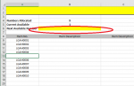
I've attached a screenshot of an example spreadsheet, where I would want the formula to go in the yellow highlighted cell (B6), and in this instance, return a value of LGAH0005, as this is the next available unique number in the list of A9-A18.

I'm absolutely open to ideas on how to do this a better way, but this is the best way I can think of to establish what your next unique available number is within a sequence at a glance.

Thank you very much in advance, this has been melting my mind so any help will be greatly received!

Best

Jimmy

 

[Giordano Bruno]

Hi Jimmy and welcome. May I suggest the following array formula?
=MIN(IF(COUNTIF(A9:A2000,"LGAH*"&ROW(A9:A2000)-ROW(A9)+1)=0,ROW(A9:A2000)-ROW(A9)+1))
Entered of course with Ctrl-Shift-Enter. (The number 2000 is arbitrary and may be extended or reduced)

 

[jasonb75]

Welcome to MrExcel

Certainly nothing broken that I can see (unless you have cross posted without informing us.

The only thing that I would suggest would be the use of XL2BB for posting examples instead of screen captures (the button on the toolbar will take you to the guide page).

the first (usually)4 digits are letters, and the next 4 are numeric.

Would all of the ID's on any one sheet have the same format and the same prefix? e.g. using your screen cap example, could there be an ID on that sheet that doesn't start with LGAH or one that has more or less than 5 numbers?

Here's a quick idea based on the example that you gave us, but it may not work with all scenarios. The prefix in B3 could be extracted from A9 using a formula if needed but I've omitted that for now.

Book1
	A	B
3	Prefix	LGAH
4	Count	9
5	Available	1
6	Next	LGAH0005
7
8	Item No.
9	LGAH0001
10	LGAH0002
11	LGAH0003
12	LGAH0004
13
14	LGAH0006
15	LGAH0007
16	LGAH0008
17	LGAH0009
18	LGAH0010
Sheet6

Cell Formulas
Range	Formula
B4	B4	=COUNTA(A9:INDEX(A:A,MATCH("zzz",A:A)))
B5	B5	=COUNTBLANK(A9:INDEX(A:A,MATCH("zzz",A:A)))
B6	B6	=B3&TEXT(SUBSTITUTE(INDEX(A:A,MATCH(TRUE,ISBLANK(A9:INDEX(A:A,B4+B5+8)),0)+8-1),B3,"")+1,"0000")
Press CTRL+SHIFT+ENTER to enter array formulas.

 

[JimmyLGS]

Giordano, Jason....thank you both for your input!

Giordano,
I tried your formula and it brought me back the numeric, without the '00' prefix, so in my example it returned '66' rather than LGAH0066. I concede this may be to do with something I did when copying the formula across to the spreadsheet, but thank you very much for your help!

Jason,
I've been a member of a few different boards and the same usually applies in that the rules are there and to be adhered to without exception (rightly so). I suppose my intention with the disclaimer was to let anyone know that if I had offended or breached a posting rule it was without malice.

And definitely no cross posting, this was my first post after creating an account. I have to say that with the very helpful responses I've had, it may not be the last!

Duly noted about XL2BB. I've tried to download it, but already struggling to find it in the add ons as it recommends in the link(?)

Concerning the ID's it absolutely is the intention that the first two letters will always be LG. In the majority of cases, the next 2 would also be letters, but we do have a very small percentage where it would only be 1 letter rather than 2. Example, LGS0001, LGS0002 or LGT0001, LGT0002 etc etc
These are rare though. The vast majority is 4 letters, 4 numbers. Perhaps in these instances, the formula for the prefix extraction you make mention of would be best.
We may also have a situation whereby the product group (LGAH for example) may contain some numbers that start LGOB, because the item may have been created as an 'odd ball' BEFORE the product group was created, if that makes sense? But in these instances, we would still want the next unique number in that product group range to be LGAH, so I assume that the newly added prefix field sorts that issue out(?)
If I can resolve the XL2BB issue, I can share a full list of the numbers and their product groups, which will give you the full idea of the structure, and which product groups will cause me problems, and how to work around them.

The black and white of the formula you have provided me is perfect, thank you! This worked when tested in a few different product groups. I've deleted some numbers in the range to test if it changes the value the way I want and it does, thank you very much for that...

I will be interested in your thoughts of a workaround for those with exceptions.

 

[jasonb75]

Jimmy,

I'll have a look at the exceptions for you a bit later on, day job is about to get in the way of forum time Looking at your example of LGS0001, etc. Would it be fair to assume always 4 numbers?

The formula should ignore the 'odd ball' numbers anyway as they don't match the expected prefix.

Looking at your example of LGS0001, etc. Would it be fair to assume always 4 numbers?

Regarding XL2BB, the add-in is not installed by default, there is an orange button the the right of the guide page (link below) where you can download it in the form of a zip file.
Once downloaded you will need to extract it to a folder where it can reside happily without being moved before adding it to excel as per the guide instructions. (Another member tried to move the extracted file after adding it to excel and had a lot of trouble getting it to work afterwards).

 

[Peter_SSs]

Welcome to the MrExcel board!

Here is another approach to consider. I have used a couple more helper cells but it should work for any length prefix or numerical part (within reason )
I have assumed data will not go beyond row 1000 but you can easily change that in the B4 formula if required.
Even if there are no blanks in the data below row 8, this will still report 1 available, my reasoning being that in such circumstance the 'next' will be whatever comes after the last entry in the list.
This will fail if cell A9 is deleted but hopefully the user would easily see that is the first available.

One further assumption is that you have the SEQUENCE function in your version of Excel 365. If not an adjustment can be made.

JimmyLGS 2020-07-28 1.xlsm
	A	B
1
2	Count	9
3	Available	1
4	Previous	LG0004
5	Prefix	LG
6	Next	LG0005
7
8	Item No.
9	LG0001
10	LG0002
11	LG0003
12	LG0004
13
14	LG0006
15	LG0007
16	LG0008
17	LG0009
18	LG0010
19
Sheet1

Cell Formulas
Range	Formula
B2	B2	=COUNTA(A:A)-COUNTA(A1:A8)
B3	B3	=MAX(COUNTBLANK(A9:INDEX(A:A,MATCH("zzz",A:A))),1)
B4	B4	=INDEX(A9:A1000,MATCH(TRUE,A9:A1000="",0)-1)
B5	B5	=LEFT(B4,AGGREGATE(15,6,FIND(SEQUENCE(10,,0),B4),1)-1)
B6	B6	=B5&TEXT(SUBSTITUTE(B4,B5,"")+1,REPT(0,LEN(B4)-LEN(B5)))

I think that we have all assumed the Item numbers will be kept neatly in order other than any deletions. That is, there is no check in mine for example that LG0005 does not already exist somewhere else in the range.

 

[Giordano Bruno]

Hi Jimmy,
You asked for the missing number, so I gave you a number. You did nothing wrong entering the formula. If you want to create the missing characters, you could add the following. I'm assuming the number formula is in cell A1
="LGAH"&REPT(0,3-INT(LOG10(A1)))&A1
Entered normally

 

[JimmyLGS]

Hi Jason

I empathise, the job is swamping me now this afternoon too in the run down the home straight to 5!

That is a fair assumption, whether the format is either 3 or 4 letters, the numeric would still be 4 digits, in the vast majority of cases.

In our existence as a company, we've made the grave mistake of allowing various people over the years to handle the fleeting of new assets, and it has cost us with some of the codings.
There may be a handful of items for example in 1 or 2 of the product groups where the number is LGBG013 or LGBG012 where (annoyingly) the user has omitted the missing 0. We have then gone on to use LGBG0013 and LGBG0012 just to confuse matters further! But thankfully, these are isolated cases, and hopefully the work around will be simple enough.

Once I'm able to share the full list with you, you'll see that we are talking exception rather than rule. with that problem.

Hope you enjoy the rest of your afternoon, and I will have a play with the XL2BB again when I get a break

Welcome to the MrExcel board!

Here is another approach to consider. I have used a couple more helper cells but it should work for any length prefix or numerical part (within reason )
I have assumed data will not go beyond row 1000 but you can easily change that in the B4 formula if required.
Even if there are no blanks in the data below row 8, this will still report 1 available, my reasoning being that in such circumstance the 'next' will be whatever comes after the last entry in the list.
This will fail if cell A9 is deleted but hopefully the user would easily see that is the first available.

One further assumption is that you have the SEQUENCE function in your version of Excel 365. If not an adjustment can be made.

JimmyLGS 2020-07-28 1.xlsm
	A	B
1
2	Count	9
3	Available	1
4	Previous	LG0004
5	Prefix	LG
6	Next	LG0005
7
8	Item No.
9	LG0001
10	LG0002
11	LG0003
12	LG0004
13
14	LG0006
15	LG0007
16	LG0008
17	LG0009
18	LG0010
19
Sheet1

Cell Formulas
Range	Formula
B2	B2	=COUNTA(A:A)-COUNTA(A1:A8)
B3	B3	=MAX(COUNTBLANK(A9:INDEX(A:A,MATCH("zzz",A:A))),1)
B4	B4	=INDEX(A9:A1000,MATCH(TRUE,A9:A1000="",0)-1)
B5	B5	=LEFT(B4,AGGREGATE(15,6,FIND(SEQUENCE(10,,0),B4),1)-1)
B6	B6	=B5&TEXT(SUBSTITUTE(B4,B5,"")+1,REPT(0,LEN(B4)-LEN(B5)))

I think that we have all assumed the Item numbers will be kept neatly in order other than any deletions. That is, there is no check in mine for example that LG0005 does not already exist somewhere else in the range.

Hi Peter

Thank you for your response. I feel I should clear something up though, because I think your formula offering will be affected by this (as Jason's has been) and it's my fault for not making it clearer in the first instance.

In my original example, the 'current available' is a bit of a red herring. It relates to data in column F which is the current 'status' of the item. This is the current status of the item on our system, be it available, on hire, scrapped, lost etc etc.

Ideally, any formula for what I want to achieve should not factor the current available field in to it. The 'Numbers allocated' field is a simple COUNTA formula that I've implemented.

For an example of how Jason's formula has been affected by this, I've just created LGBL product group sheet, and there are only two items on there LGBL0001 & LGBL0002.
So, in the 'Next' field, this should ideally be showing me LGBL0003 but I get the #N/A using Jason's formula, and I am sure it is because the 'current available' is 0, owing to the fact that both the items are currently showing 'in service' in column F. 'Current Available' is currently running on a COUNTIF function that I've added to return a value where 'Available' is showing.

As for the tidiness of the numbers that is a fair assumption, and in most instances they are tidy. I've mentioned a few anomalies in my response to Jason, but thankfully these are the exception.

In its most simplistic terms what I am hoping to achieve is that if I have a list of 0001-0150 in column A (with a varying alphabetic 3or4 digit sequence at the beginning which will always start LG) I would like a cell (Next, B6) to tell me what is the next available number in that sequence. If there are gaps in the sequence, it would be the next number in the sequence for the first blank. If there are no gaps in the sequence, it would show LGxx0151, in this example, as there are no gaps and the next in the sequence will be 0151.

Ideally, the formula needs to be adaptable easily enough when creating the next sheet, as I am using 'move or copy' on the previous sheet and selecting (move to end) & 'create copy'.

Hopefully that makes sense, and will save any more confusion

Thank you all so far

Jimmy

 

[Peter_SSs]

I've just created LGBL product group sheet, and there are only two items on there LGBL0001 & LGBL0002.
So, in the 'Next' field, this should ideally be showing me LGBL0003

.. and that is what my suggestion does. Can you give examples of where/how it fails so that I can try and correct if there is a problem.
My suggestion does not use the 'Available' value it is just there because you had it.

JimmyLGS 2020-07-28 1.xlsm
	A	B
1
2	Count	2
3	Available	1
4	Previous	LGBL0002
5	Prefix	LGBL
6	Next	LGBL0003
7
8	Item No.
9	LGBL0001
10	LGBL0002
11
12
LGBL

Cell Formulas
Range	Formula
B2	B2	=COUNTA(A:A)-COUNTA(A1:A8)
B3	B3	=MAX(COUNTBLANK(A9:INDEX(A:A,MATCH("zzz",A:A))),1)
B4	B4	=INDEX(A9:A1000,MATCH(TRUE,A9:A1000="",0)-1)
B5	B5	=LEFT(B4,AGGREGATE(15,6,FIND(SEQUENCE(10,,0),B4),1)-1)
B6	B6	=B5&TEXT(SUBSTITUTE(B4,B5,"")+1,REPT(0,LEN(B4)-LEN(B5)))

 

[JimmyLGS]

.. and that is what my suggestion does. Can you give examples of where/how it fails so that I can try and correct if there is a problem.
My suggestion does not use the 'Available' value it is just there because you had it.

JimmyLGS 2020-07-28 1.xlsm
	A	B
1
2	Count	2
3	Available	1
4	Previous	LGBL0002
5	Prefix	LGBL
6	Next	LGBL0003
7
8	Item No.
9	LGBL0001
10	LGBL0002
11
12
LGBL

Cell Formulas
Range	Formula
B2	B2	=COUNTA(A:A)-COUNTA(A1:A8)
B3	B3	=MAX(COUNTBLANK(A9:INDEX(A:A,MATCH("zzz",A:A))),1)
B4	B4	=INDEX(A9:A1000,MATCH(TRUE,A9:A1000="",0)-1)
B5	B5	=LEFT(B4,AGGREGATE(15,6,FIND(SEQUENCE(10,,0),B4),1)-1)
B6	B6	=B5&TEXT(SUBSTITUTE(B4,B5,"")+1,REPT(0,LEN(B4)-LEN(B5)))

Peter I confess, I wrongly assumed that your offering relied also on the available status and didn't even try it, apologies.

I've now tried your formulas, and it looks as though that has worked a dream, thanks so much!!! 6 groups down, only another 74 to go.....Fancy creating a macro that will do it all for me?! lol

@Jason, you can save yourself the heartache after your shift now! Thank you very much for your help also

A very positive first experience on the forum, and will absolutely post again

Thank you all

Jimmy