Return the end time for a person ba looking at the start time for another task

Tempt

New Member
Joined
Aug 15, 2019
Messages
6
Hi, everyone.

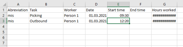
I have a table of people with a date, start time and end time, as well as task performed by that person. The problem is that most cells in the colum of end time are blank and I would like to take the start time of that person on the same day for another task (the person changed the task but didn't enter the end time).

Now I am trying to figure out how to return the end time for the same person on the same date for a different task when he/she changes it where I define the end time as the start time for the same day and person but a different task.

My table looks as follows.

What I want is a formula in column F to return the end time defined as a start time for a different task for the same person on the same day (here the value in cell E3). Alternatively I could do it in another sheet where I could match the corresponding value, which I also can't figure out.

Any help and tip would be much appreciated.
 

Attachments

  • Unbenannt9999.PNG
    Unbenannt9999.PNG
    9.8 KB · Views: 8

Excel Facts

Excel Wisdom
Using a mouse in Excel is the work equivalent of wearing a lanyard when you first get to college
Hi Tempt,

Can I assume the data is in ascending date/time sequence?
 
Upvote 0
As some End Times are entered then you'll need an extra column for the Calculate End Time, being the entered time or next for that day for that worker.

If you've no following time for an entry then I show "No end time" though you may want to force it to normal clocking off time.

Tempt.xlsx
ABCDEFGH
1AbbreviationTaskWorkerDateStart TimeEnd TimeCalculated End TimeHours Worked
2MISPickingWorker103-Jan-219:3010:301:00
3MISPackingWorker103-Jan-2110:3011:301:00
4TTEParkingWorker103-Jan-2111:3012:301:00
5JKLPortingWorker103-Jan-2112:30No end time 
6MISPickingWorker503-Jan-219:3010:301:00
7TTEPackingWorker503-Jan-2110:3016:4516:456:15
8JKLParkingWorker504-Jan-2111:4412:300:46
9MISPortingWorker504-Jan-2112:30No end time 
10TTEPickingWorker104-Jan-219:3010:301:00
11JKLPackingWorker104-Jan-2110:3011:301:00
12MISParkingWorker104-Jan-2111:3012:301:00
13TTEPortingWorker104-Jan-2112:3017:0017:004:30
Sheet1
Cell Formulas
RangeFormula
G2:G13G2=IF(F2="",IFERROR(INDEX($E$2:$E$9995,AGGREGATE(15,6,ROW($E$2:$E$9995)-ROW($E$1)/(($C$2:$C$9995=C2)*($D$2:$D$9995=D2)*(ROW($E$2:$E$9995)>ROW(E2))),1)),"No end time"),F2)
H2:H13H2=IFERROR(G2-E2,"")
Hey, thanks for the answer. Could you please explain what the formula does?
 
Upvote 0
If and End Time was entered then use it.
=IF(F2="",...F2)

If the AGGREGATE fails (it gives a #NUM error if no cases are found) then no matching next job was found.
IFERROR(...,"No end time")

Retrieve the Start Time
INDEX($E$2:$E$9995,...)

AGGREGATE is using the SMALL function (15) and ignoring internal errors. The ROW means it's not looking into each cell of $E$2:$E$9995 but rather looking at every row from 2 to 9995 so we must subtract the heading row to get the actual row number.
The 1 at the end is because it can get the first, second, third, etc. but in this case we only want the first, so 1.
AGGREGATE(15,6,ROW($E$2:$E$9995)-ROW($E$1)...,1)

Now for every row number we divide it by the logicalresult of three comparisons. If any is FALSE (zero) then multiplied together will always be zero and divided into the row number will give #DIV/0 which the option 6 of AGGREGATE ignores.
/

So for each row of C, D and E 2 to 9995 it checks if they equal the current C or D (if so then we have the same Worker and Date) and if the row being looked at is greater than the current row (so we don't get an earlier time or time of the current row).
(($C$2:$C$9995=C2)*($D$2:$D$9995=D2)*(ROW($E$2:$E$9995)>ROW(E2)))
Hey, thank you very much. It works.
 
Upvote 0

Forum statistics

Threads
1,214,810
Messages
6,121,690
Members
449,048
Latest member
81jamesacct

We've detected that you are using an adblocker.

We have a great community of people providing Excel help here, but the hosting costs are enormous. You can help keep this site running by allowing ads on MrExcel.com.
Allow Ads at MrExcel

Which adblocker are you using?

Disable AdBlock

Follow these easy steps to disable AdBlock

1)Click on the icon in the browser’s toolbar.
2)Click on the icon in the browser’s toolbar.
2)Click on the "Pause on this site" option.
Go back

Disable AdBlock Plus

Follow these easy steps to disable AdBlock Plus

1)Click on the icon in the browser’s toolbar.
2)Click on the toggle to disable it for "mrexcel.com".
Go back

Disable uBlock Origin

Follow these easy steps to disable uBlock Origin

1)Click on the icon in the browser’s toolbar.
2)Click on the "Power" button.
3)Click on the "Refresh" button.
Go back

Disable uBlock

Follow these easy steps to disable uBlock

1)Click on the icon in the browser’s toolbar.
2)Click on the "Power" button.
3)Click on the "Refresh" button.
Go back
Back
Top