Return Value Based on Multiple Criteria

[KMorrison12345]

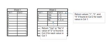
I have a file that lists multiple values for each item. I am trying to get the data so that each item has only one row. However, not every item has every value. I wish I could give access to the actual data but it is sensitive so I created an image to explain what result I am looking for. I am trying to avoid using certain vocabulary because I believe I have been looking to the wrong formulas to achieve this.

Essentially, for items listed in column 1 on the first sheet, they have one value per row. I would like each item to have only one row on the second sheet. However, not all items have the same value in col 2, but sometimes they do.
In the image, I would like in Sheet 2, Col 2 to list a yes or no if Sheet 1, Col 2 contains the number "2". And in Sheet 2, Col 3 to list out each number for numbers 1, 3, and 4 if they are available for an item. In the example provided, only item C has the value 4, therefore it is written out in Col 3 for item C only.

I hope this makes sense. I will be back on tomorrow morning to check.

 

[Z51]

Assuming:
Table on Sheet1 is in A:B (A1:B1 has headers, row 2 is first data row)
Table on Sheet2 is in A:C (A1:C1 has headers, row 2 is first data row)

In Sheet2!B2, use this formula and fill down:

=IF(COUNTIFS(Sheet1!A:A,A2,Sheet1!B:B,2)>0,"Yes","No")

In Sheet2!C2, use this formula and fill down:

=TEXTJOIN(", ",TRUE,IF(ISNUMBER(MATCH(A2&"1",Sheet1!$A$1:$A$20&Sheet1!$B$1:$B$20,0)),1,""),IF(ISNUMBER(MATCH(A2&"3",Sheet1!$A$1:$A$20&Sheet1!$B$1:$B$20,0)),3,""),IF(ISNUMBER(MATCH(A2&"4",Sheet1!$A$1:$A$20&Sheet1!$B$1:$B$20,0)),4,""))

Adjust your source data range in the last formula from rows 1:20 to a larger range that encompasses all of your rows. Hopefully it's not 500,000 rows.

 

[Fluff]

Another option

Fluff.xlsm
	A	B	C	D	E	F	G	H
1
2	a	1				a	Yes	1, 3
3	a	2				b	Yes	1, 3
4	a	3				c	No	1, 3, 4
5	b	1
6	b	2
7	b	3
8	c	1
9	c	3
10	c	4
Sheet1

Cell Formulas
Range	Formula
G2:G4	G2	=IF(COUNTIFS(A:A,F2,B:B,2),"Yes","No")
H2:H4	H2	=TEXTJOIN(", ",,IF(($A$2:$A$10=F2)*(($B$2:$B$10=1)+($B$2:$B$10=3)+($B$2:$B$10=4)),$B$2:$B$10,""))
Press CTRL+SHIFT+ENTER to enter array formulas.

 

[KMorrison12345]

Assuming:
Table on Sheet1 is in A:B (A1:B1 has headers, row 2 is first data row)
Table on Sheet2 is in A:C (A1:C1 has headers, row 2 is first data row)

In Sheet2!B2, use this formula and fill down:

=IF(COUNTIFS(Sheet1!A:A,A2,Sheet1!B:B,2)>0,"Yes","No")

In Sheet2!C2, use this formula and fill down:

=TEXTJOIN(", ",TRUE,IF(ISNUMBER(MATCH(A2&"1",Sheet1!$A$1:$A$20&Sheet1!$B$1:$B$20,0)),1,""),IF(ISNUMBER(MATCH(A2&"3",Sheet1!$A$1:$A$20&Sheet1!$B$1:$B$20,0)),3,""),IF(ISNUMBER(MATCH(A2&"4",Sheet1!$A$1:$A$20&Sheet1!$B$1:$B$20,0)),4,""))

Adjust your source data range in the last formula from rows 1:20 to a larger range that encompasses all of your rows. Hopefully it's not 500,000 rows.

The first formula worked like a charm. The second one returns blank cells. This is the adjustment I made to match my file

=TEXTJOIN(", ",TRUE,IF(ISNUMBER(MATCH(A3,District!A:A&District!L:L,0)),1,""),IF(ISNUMBER(MATCH(A3&"6",District!A:A&District!L:L,0)),6,""),IF(ISNUMBER(MATCH(A3&"8",District!A:A&District!L:L,0)),8,""))

District is the name of the sheet I am pulling data from. I am looking for the numbers 1, 6 and/or 8 in column L