mike4president
New Member
- Joined
- May 1, 2021
- Messages
- 2
- Office Version
- 365
- Platform
- Windows
Hello,
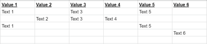
I'm trying to create a relative ranking structure based on cell values within a repeating range.
I have ranked the text values accordingly.

I then have a sheet with columns that contain subsets of these text values like so;

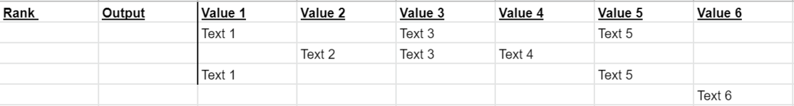
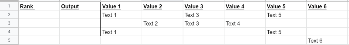
What I am trying to accomplish, is that when a Rank of 1 is entered into a cell in row A, it will return the highest value of that row based on the column values in row B. So as an example;
If 1 was entered into cell A2, it would return "Text 1" in B2. If 2 was entered in A2 it would return "Text 3" in B2. If 3 was entered in A2 it would return "text 5". If any other rank (4-20) was entered B2 would remain blank. The same would happen in Row 3 except it would consider "Text 2" as rank 1, "Text 3" as rank 2, and "Text 4" as rank 3.
I can't seem to get this to work properly with any combination of COUNTIF or Rank, any help here would be extremely appreciated!
I'm trying to create a relative ranking structure based on cell values within a repeating range.
I have ranked the text values accordingly.
I then have a sheet with columns that contain subsets of these text values like so;
What I am trying to accomplish, is that when a Rank of 1 is entered into a cell in row A, it will return the highest value of that row based on the column values in row B. So as an example;
If 1 was entered into cell A2, it would return "Text 1" in B2. If 2 was entered in A2 it would return "Text 3" in B2. If 3 was entered in A2 it would return "text 5". If any other rank (4-20) was entered B2 would remain blank. The same would happen in Row 3 except it would consider "Text 2" as rank 1, "Text 3" as rank 2, and "Text 4" as rank 3.
I can't seem to get this to work properly with any combination of COUNTIF or Rank, any help here would be extremely appreciated!