Returning average value under specific conditions

[bl3s]

Hi,

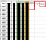
I have a large spreadsheet with loads of data.
First, I'd like to give you a little idea what is the spreadsheet used for, so you get understanding what do I really need to calculate.
I do run injection moulder, making some product. Each 'female' produces some values in 'performance' columns, however values vary slightly depending on with which axis a female is paired to.
Axises generally can be grouped into 3 that perform similarly:
1)10, 20, 30, 150, 160, 170, 180
2)40,50,130,140
3)70,80,90,100,110,120

I need to calculate average value achieved by each female in 'performance' column but for specific groups of axis, in other words I need to calculate 3 different averages for the same 'female' and return these next to appropriate cell in 'inventory' tab. In the 'performance' column there are blank cells (these come from the past) and some text values (N/A, #N/A or SPR). Sheet is getting bigger as every new batch results get into it.

I tried to use index/match, if, average in various combinations, but I did not achieve any positive results.
If something sounds unclear, I will try to explain it better.
Many thanks for your help

 

[Toadstool]

Hi BL3s,

You could add a column to identify the group then just use AVERAGEIFS

Book1
	E	F	G									P	Q	R									AA	AB	AC	AD
1	Axis	Female	Group										Performance										Female	10/20/30/150/160/170/180	40/50/130/140	70/80/90/100/110/120
2	170	SH2	1										1										SH2	3.5	2.5	4.5
3	140	SH2	2										2										SH3		7
4	40	SH2	2										3										SH4			8
5	120	SH2	3										4
6	90	SH2	3										5
7	10	SH2	1										6
8	130	SH3	2										7
9	110	SH4	3										8
Sheet1

Cell Formulas
Range	Formula
AB2:AD4	AB2	=IFERROR(AVERAGEIFS($Q$2:$Q$9,$F$2:$F$9,$AA2,$G$2:$G$9,COLUMN()-COLUMNS($A2:$AA2)),"")
G2:G9	G2	=MATCH("*"&E2&"*",$AB$1:$AD$1,0)

 

[bl3s]

Hi Toadstool,

Many thanks for your attention.
I have tried to implement your solution, however when I extended the ranges, aferageifs simply does not show anything. Any idea?

 

[Peter_SSs]

I have tried to implement your solution, however when I extended the ranges, aferageifs simply does not show anything. Any idea?

I suspect it is to do with using different columns or that you have some error values among your data.

Using Toadstool's layout & data, you could try this slightly simplified version of that formula & see if you can adapt that better. The 'COLUMNS' part of the formula should have an absolute column reference for the first instance of the first column that contains these formulas.

Note also that I have changed the column G formula. As it was, it could put rows into the incorrect group (eg change one of the column E values to 50 and you will see that the original column G formula returns Group 1 when it should be Group 2)

20 07 02.xlsm
	E	F	G										Q	R									AA	AB	AC	AD
1	Axis	Female	Group										Performance										Female	10/20/30/150/160/170/180	40/50/130/140	70/80/90/100/110/120
2	170	SH2	1										1										SH2	3.5	2.5	4.5
3	140	SH2	2										2										SH3		7
4	40	SH2	2										3										SH4			8
5	120	SH2	3										4
6	90	SH2	3										5
7	10	SH2	1										6
8	130	SH3	2										7
9	110	SH4	3										8
Average 1

Cell Formulas
Range	Formula
AB2:AD4	AB2	=IFERROR(AVERAGEIFS($Q$2:$Q$9,$F$2:$F$9,$AA2,$G$2:$G$9,COLUMNS($AB2:AB2)),"")
G2:G9	G2	=MATCH("*/"&E2&"/*","/"&$AB$1:$AD$1&"/",0)

As an alternative, you could also try this formula that does not require the helper column.

20 07 02.xlsm
	E	F	G										Q	R									AA	AB	AC	AD
1	Axis	Female											Performance										Female	10/20/30/150/160/170/180	40/50/130/140	70/80/90/100/110/120
2	170	SH2											1										SH2	3.5	2.5	4.5
3	140	SH2											2										SH3		7
4	40	SH2											3										SH4			8
5	120	SH2											4
6	90	SH2											5
7	10	SH2											6
8	130	SH3											7
9	110	SH4											8
Average 2

Cell Formulas
Range	Formula
AB2:AD4	AB2	=IFERROR(SUMPRODUCT(--($F$2:$F$9=$AA2),--(ISNUMBER(SEARCH("/"&$E$2:$E$9&"/","/"&AB$1&"/"))),$Q$2:$Q$9)/SUMPRODUCT(--($F$2:$F$9=$AA2),--(ISNUMBER(SEARCH("/"&$E$2:$E$9&"/","/"&AB$1&"/")))),"")

 

[bl3s]

Hi,

@Peter_SSs I have encountered the same issue as with @Toadstool solution- no value returned.

As for grouping the axises I found the best result with index and match, see below

#Config builder STM- new1.xlsx
	E	F	G	H	I	J				N	O	P	Q	R	S	T	U	V	W	X	Y	Z	AA	AB	AC	AD
1	Axis	Female Insert		abc	Male Insert	pcd				a	b	c	performance	Hit/Miss	Miss	Hit %	65.23%	Female Available	Male Available	Row number				10/20/30/150/160/170/180	40/50/130/140	60/70/80/90/100/110/120
2	170	SHT9/37	1	SHT9FPM/26	S9C-2.87/19	SHT9MP/25				-3.00	-2.25	170		Miss	3754	7042		Available	Available	1	1	10	SHT9/37
3	170	SHT9/40	1	SHT9FPM/27	S9C-2.87/28	SHT9MP/26				-3.50	-2.25	170		Hit				Available	Available	2	1	20	SHT9/40
4	170	SHT9/60	1	SHT9FPM/28	S9C-2.87/27	SHT9MP/27				-5.75	-2.25	170		Hit				Available	Available	3	1	30	SHT9/103
5	10	SHT9/165	1	SHT9FPM/29	S9C-2.87/32	SHT9MP/28				-7.00	-2.25	10		Hit				Available	Available	4	2	40	SHT9/104
6	160	SHT9/82	1	SHT9FPM/30	S9C-2.87/8	SHT9MP/29				-8.00	-2.25	160		Hit				Available	Available	5	2	50	SHT9/105
7	180	SHT9/182	1	SHT9FPM/31	S9C-2.87/30	SHT9MP/30				-8.50	-2.25	180		Hit				Available	#N/A	6	3	60	SHT9/106
8	150	SHT9/131	1	SHT9FPM/32	S9C-2.87/6	SHT9MP/31				#N/A	#N/A	#N/A		#N/A				#N/A	Available	7	3	70	SHT9/107
9	30	SHT9/41	1	SHT9FPM/33	S9C-2.87/5	SHT9MP/32				-3.75	-2.25	30		Hit				Available	Available	8	3	80	SHT9/108
10	10	SHT9/65	1	SHT9FPM/34	S9C-2.87/33	SHT9MP/33				-6.00	-2.25	10		Miss				Available	Available	9	3	90	SHT9/109
11	70	SHT9/309	3	SHT9FPM/35	S9C-2.12/36	SHT9MP/34				-7.50	-2.25	70		Hit				Available	Available	10	3	100	SHT9/110
12	180	SHT9/305	1	SHT9FPM/36	S9C-2.87/11	SHT9MP/35				-8.50	-2.25	180		Miss				Available	#N/A	11	3	110	SHT9/111
13	180	SHT9/183	1	SHT9FPM/37	S9C-2.87/13	SHT9MP/36				-8.50	-2.25	180		Hit				Available	Available	12	3	120	SHT9/112
14	30	SHT9/116	1	SHT9FPM/26	S9C-2.12/42	SHT9MP/25				-1.25	-1.75	30		Hit				Available	Available	13	2	130	SHT9/113
15	150	SHT9/103	1	SHT9FPM/27	S9C-2.12/30	SHT9MP/26				-2.25	-1.75	150		Hit				Available	Available	14	2	140	SHT9/114
16	170	SHT9/39	1	SHT9FPM/28	S9C-2.12/33	SHT9MP/27				-3.50	-1.75	170		Hit				Available	Available	15	1	150	SHT9/115
17	40	SHT9/44	2	SHT9FPM/29	S9C-1.87/1	SHT9MP/28				-3.75	-1.75	40		Hit				Available	Available	16	1	160	SHT9/115
18	140	SHT9/107	2	SHT9FPM/30	S9C-1.87/5	SHT9MP/29				-4.25	-1.75	140		Hit				Available	Available	17	1	170
19	20	SHT9/120	1	SHT9FPM/32	S9C-2.12/40	SHT9MP/31				-1.75	-1.75	20		Hit				#N/A	Available	18	1	180
STM data tab

Cell Formulas
Range	Formula
U1	U1	=T2/(T2+S2)
S2	S2	=COUNTIF(R2:R29996,"Miss")
T2	T2	=COUNTIF(R2:R30048,"HIT")
V2:V19	V2	=IF(INDEX('Insert Inventory'!A:A,(MATCH(F2,'Insert Inventory'!A:A,0)))>1,"Available","Not Available")
W2:W19	W2	=IF(INDEX('Insert Inventory'!K:K,(MATCH(I2,'Insert Inventory'!K:K,0)))>1,"Available","Not Available")
AB3:AD3,AC2:AD2	AC2	=IFERROR(AVERAGEIFS($Q$2:$Q$15009,$F$2:$F$15009,$AA2,$G$2:$G$15009,COLUMN()-COLUMNS($A2:$AA2)),"")
G2:G19	G2	=INDEX($Y$2:$Y$19,(MATCH(E:E,$Z$2:$Z$19,0)))
R2:R19	R2	=IF(AND(N2=D2,O2=C2,P2=E2),"Hit","Miss")

Named Ranges
Name	Refers To	Cells
'Insert Inventory'!_FilterDatabase	='Insert Inventory'!$A$1:$R$498	V2:V19

Cells with Conditional Formatting
Cell	Condition		Cell Format	Stop If True
N:P	Cell Value	contains "SPR"	text	NO
V1:W12157	Cell Value	not containing "Available"	text	NO

in cell AA3 I left your formula with extended range. I hope I haven't done silly mistake when implementing it into the sheet.

 

[Peter_SSs]

Hi,

@Peter_SSs I have encountered the same issue as with @Toadstool solution- no value returned.


in cell AA3 I left your formula with extended range. I hope I haven't done silly mistake when implementing it into the sheet.

That is not my formula in AA3.

Never-the-less, it appears to me that you are not getting any results because the AVERAGEIFS function in that formula is trying to average values in column Q. Since there are no values in column Q, that will result in a #DIV/0! error and hence the IFERROR wrapped around that function returns ""

 

[bl3s]

Hi @Peter_SSs

Thank you for your reply.
So apparently... Formulas work. I implemented them next to an old insert that no longer exists in my inventory due to being scrapped and there were no values in performance columns as I started collecting these data recently, hence no output in cells.
Thank you very much for your help!

 

[Peter_SSs]

You're welcome. Glad you got it resolved.