Returning employee status based on client

[GREGRACH]

Hi Everyone,
Firstly, thanks for reading my question.
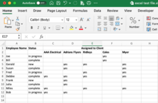
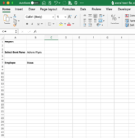
I have a spreadsheet that lists employee names, their status and the clients they are assigned to. I am trying to create a separate sheet to create a report to send to clients that lists the employees that are assigned to them and their status. I'm not sure if I should be using vlookup or a pivot table or something else? I'm sure there is a simple answer but I'm having no luck. I've attached some image examples.
Any help would be hugely appreciated!
Thank you

* I should add that in the report, the 'select client name' is a data validation dropdown list.

 

[alansidman]

1. What version of excel are you using? Please update your profile so that we can tailor a solution.
2. We cannot manipulate data in a picture. Please update your question with sample data using the XL2BB function provided in this forum.

 

[GREGRACH]

1. What version of excel are you using? Please update your profile so that we can tailor a solution.
2. We cannot manipulate data in a picture. Please update your question with sample data using the XL2BB function provided in this forum.

Apologies. Attached.

excel test file.xlsx
	A	B	C	D	E	F	G
1	Employee Name	Status	Assigned to Client
2			AAA Electrical	Adrians Flyers	Ridleys	Coles	Myer
3	Joe	in progress				yes
4	Bill	complete				yes
5	Gerald	new		yes	yes		yes
6	Susan	complete		yes			yes
7	Fred	in progress			yes		yes
8	Debbie	complete	yes	yes	yes		yes
9	Frank	new		yes
10	Julia	complete		yes
11	Miles	complete	yes		yes		yes
12	Bob	in progress	yes	yes
13
Employee Status

Cells with Data Validation
Cell	Allow	Criteria
B3:B12	List	='Data Validation lists'!$A$1:$A$3
C3:G12	List	='Data Validation lists'!$B$1:$B$3

excel test file.xlsx
	A	B	C
1	Report
2
3
4	Select Client Name	Adrians Flyers
5
6
7	Employee	Status
8
9
10
11
12
13
14
15
16
17
18
19
20
21
22
23
24
25
26
27
28
29
30
31
32
33
Client Form

Cells with Data Validation
Cell	Allow	Criteria
B4	List	='Employee Status'!$C$2:$G$2

 

[GREGRACH]

1. What version of excel are you using? Please update your profile so that we can tailor a solution.
2. We cannot manipulate data in a picture. Please update your question with sample data using the XL2BB function provided in this forum.

Thank you. I have updated everything. Thanks for replying.

 

[alansidman]

My apologies, but I am unable to assist you as my solution requires a Windows Operating System. I would use Power Query, but unfortunately this is not an option for you as it not available for MAC operating systems. Good Luck.

 

[Alex Blakenburg]

My apologies, but I am unable to assist you as my solution requires a Windows Operating System. I would use Power Query, but unfortunately this is not an option for you as it not available for MAC operating systems. Good Luck.

The OP has 365 it should have PQ
Import data in Excel for Mac (Power Query)

 

[alansidman]

Thanks Alex, it was my understanding that PQ had not been added to 365 for MAC.

Note to OP: Heading out for a Hike in the Rockies. Will check back later and give you Mcode if no one has offered up a solution by the time I return.

 

[alansidman]

Here is the Mcode for a Power Query Solution

let
    Source = Excel.CurrentWorkbook(){[Name="Table1"]}[Content],
    #"Changed Type" = Table.TransformColumnTypes(Source,{{"Employee Name", type text}, {"Status", type text}, {"AAA Electrical", type text}, {"Adrians Flyers", type text}, {"Ridleys", type text}, {"Coles", type text}, {"Myer", type text}}),
    #"Unpivoted Other Columns" = Table.UnpivotOtherColumns(#"Changed Type", {"Employee Name", "Status"}, "Attribute", "Value"),
    #"Removed Columns" = Table.RemoveColumns(#"Unpivoted Other Columns",{"Status", "Value"}),
    #"Grouped Rows" = Table.Group(#"Removed Columns", {"Attribute"}, {{"Data", each _, type table [Employee Name=nullable text, Attribute=text]}}),
    #"Added Custom" = Table.AddColumn(#"Grouped Rows", "Custom", each Table.AddIndexColumn([Data],"Index",1,1)),
    #"Removed Columns1" = Table.RemoveColumns(#"Added Custom",{"Data"}),
    #"Expanded Custom" = Table.ExpandTableColumn(#"Removed Columns1", "Custom", {"Employee Name", "Index"}, {"Employee Name", "Index"}),
    #"Pivoted Column" = Table.Pivot(Table.TransformColumnTypes(#"Expanded Custom", {{"Index", type text}}, "en-US"), List.Distinct(Table.TransformColumnTypes(#"Expanded Custom", {{"Index", type text}}, "en-US")[Index]), "Index", "Employee Name")
in
    #"Pivoted Column"

Book13
	A	B	C	D	E	F	G
2	Employee Name	Status	AAA Electrical	Adrians Flyers	Ridleys	Coles	Myer
3	Joe	in progress				yes
4	Bill	complete				yes
5	Gerald	new		yes	yes		yes
6	Susan	complete		yes			yes
7	Fred	in progress			yes		yes
8	Debbie	complete	yes	yes	yes		yes
9	Frank	new		yes
10	Julia	complete		yes
11	Miles	complete	yes		yes		yes
12	Bob	in progress	yes	yes
13
14	Attribute	1	2	3	4	5	6
15	AAA Electrical	Debbie	Miles	Bob
16	Adrians Flyers	Gerald	Susan	Debbie	Frank	Julia	Bob
17	Coles	Joe	Bill
18	Myer	Gerald	Susan	Fred	Debbie	Miles
19	Ridleys	Gerald	Fred	Debbie	Miles
20
Sheet1

 

[GREGRACH]

Here is the Mcode for a Power Query Solution

let
    Source = Excel.CurrentWorkbook(){[Name="Table1"]}[Content],
    #"Changed Type" = Table.TransformColumnTypes(Source,{{"Employee Name", type text}, {"Status", type text}, {"AAA Electrical", type text}, {"Adrians Flyers", type text}, {"Ridleys", type text}, {"Coles", type text}, {"Myer", type text}}),
    #"Unpivoted Other Columns" = Table.UnpivotOtherColumns(#"Changed Type", {"Employee Name", "Status"}, "Attribute", "Value"),
    #"Removed Columns" = Table.RemoveColumns(#"Unpivoted Other Columns",{"Status", "Value"}),
    #"Grouped Rows" = Table.Group(#"Removed Columns", {"Attribute"}, {{"Data", each _, type table [Employee Name=nullable text, Attribute=text]}}),
    #"Added Custom" = Table.AddColumn(#"Grouped Rows", "Custom", each Table.AddIndexColumn([Data],"Index",1,1)),
    #"Removed Columns1" = Table.RemoveColumns(#"Added Custom",{"Data"}),
    #"Expanded Custom" = Table.ExpandTableColumn(#"Removed Columns1", "Custom", {"Employee Name", "Index"}, {"Employee Name", "Index"}),
    #"Pivoted Column" = Table.Pivot(Table.TransformColumnTypes(#"Expanded Custom", {{"Index", type text}}, "en-US"), List.Distinct(Table.TransformColumnTypes(#"Expanded Custom", {{"Index", type text}}, "en-US")[Index]), "Index", "Employee Name")
in
    #"Pivoted Column"

Book13
	A	B	C	D	E	F	G
2	Employee Name	Status	AAA Electrical	Adrians Flyers	Ridleys	Coles	Myer
3	Joe	in progress				yes
4	Bill	complete				yes
5	Gerald	new		yes	yes		yes
6	Susan	complete		yes			yes
7	Fred	in progress			yes		yes
8	Debbie	complete	yes	yes	yes		yes
9	Frank	new		yes
10	Julia	complete		yes
11	Miles	complete	yes		yes		yes
12	Bob	in progress	yes	yes
13
14	Attribute	1	2	3	4	5	6
15	AAA Electrical	Debbie	Miles	Bob
16	Adrians Flyers	Gerald	Susan	Debbie	Frank	Julia	Bob
17	Coles	Joe	Bill
18	Myer	Gerald	Susan	Fred	Debbie	Miles
19	Ridleys	Gerald	Fred	Debbie	Miles
20
Sheet1

Thanks so much for taking the time to provide a solution. Apologies I didn't reply sooner. I didn't get a notification you had replied so have only just checked. Thanks again!