Returning only visible data for RANDARRAY

[baileyb103]

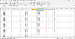
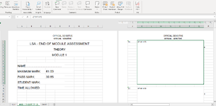
Hi. I am creating a question bank for a module that is made up of multiple class studies. I have created the full question bank and I am using RANDARRAY function to return a random test paper. Initially I just wanted to create an end of module test but now I've been asked if I can use the bank to create random tests for each class study. I have attempted this by adding in a column with the class study number for each question and filtering, but the RANDARRAY returns results from all the data not just the visible data. Is there anything I can add to the formula or do to the sheet to only return data from the visible cells? The current formula looks like this... =INDEX(SORTBY(C2:F118,RANDARRAY(ROWS(C2:F118))),SEQUENCE(H1),{1,2,3,4})

 

[jasonb75]

Personally I would add a helper column to the question bank using the formula

=SUBTOTAL(3,C2)

filled down to the end, then use that as the first array in SORTBY.

Note that the SUBTOTAL formula needs to look at a column that will have data in all visible rows, formula blanks are ok but empty cells will mess up the sort order.

Assuming the helper formula in G2:G118 you would then change your formula to

=INDEX(SORTBY(C2:G118,G2:G118,-1,RANDARRAY(ROWS(C2:F118))),SEQUENCE(H1),{1,2,3,4})

I haven't got anything to hand that is suitable to test this on but I believe that it will work as required.

 

[baileyb103]

Thank you Jason. I've tried that but there is an error box comes up saying I've entered too few arguments for this function.

 

[jasonb75]

Sorry, I forgot to include the sort order for the second array in SORTBY.

=INDEX(SORTBY(C2:G118,G2:G118,-1,RANDARRAY(ROWS(C2:F118)),1),SEQUENCE(H1),{1,2,3,4})

 

[Fluff]

Another option, still using the helper column in G is

=LET(f,FILTER(C2:F118,G2:G118=1),TAKE(SORTBY(f,RANDARRAY(ROWS(f))),H1))

 

[baileyb103]

Sorry, I forgot to include the sort order for the second array in SORTBY.

=INDEX(SORTBY(C2:G118,G2:G118,-1,RANDARRAY(ROWS(C2:F118)),1),SEQUENCE(H1),{1,2,3,4})

That now works perfectly thank you.

 

[baileyb103]

Another option, still using the helper column in G is

=LET(f,FILTER(C2:F118,G2:G118=1),TAKE(SORTBY(f,RANDARRAY(ROWS(f))),H1))

Unfortunately this didn't work. The one that Jason put in now does so just going to go with that, but thank you anyway.

 

[jasonb75]

@Fluffs formula should give the desired output, it might be that you don't have the update with the TAKE function yet.

 

[baileyb103]

Good afternoon, I thought this had worked but it doesn't seem to be now. I have made the spreadsheet so I can share it (ie no sensitive questions). When I filter the columns for say user group 1, the test paper on the other tab still shows questions from the unfiltered list.

 

[Fluff]

In what way didn't the formula I suggested work?