Score Matching

[Proezas]

Hello!

I've been trying and searching about it for hours and can't find a solution. I do have 2 sheets of information - one of them gives me a whole plan of scores - divided by category and results with a score for each possible result. The other gives me the information of the individuals.

I want a formula that finds the category, then, in that row, finds the result and then gives the right score - I can use a thousand IFs and make it work, but I want to find a simpler way (my excel is 2007, so I don't have IFS formula that could have helped).

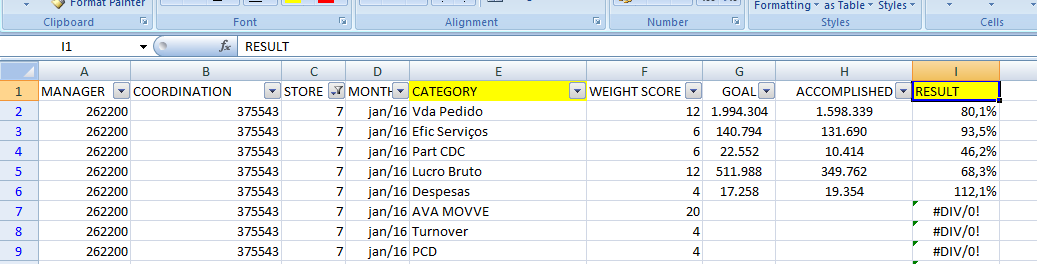
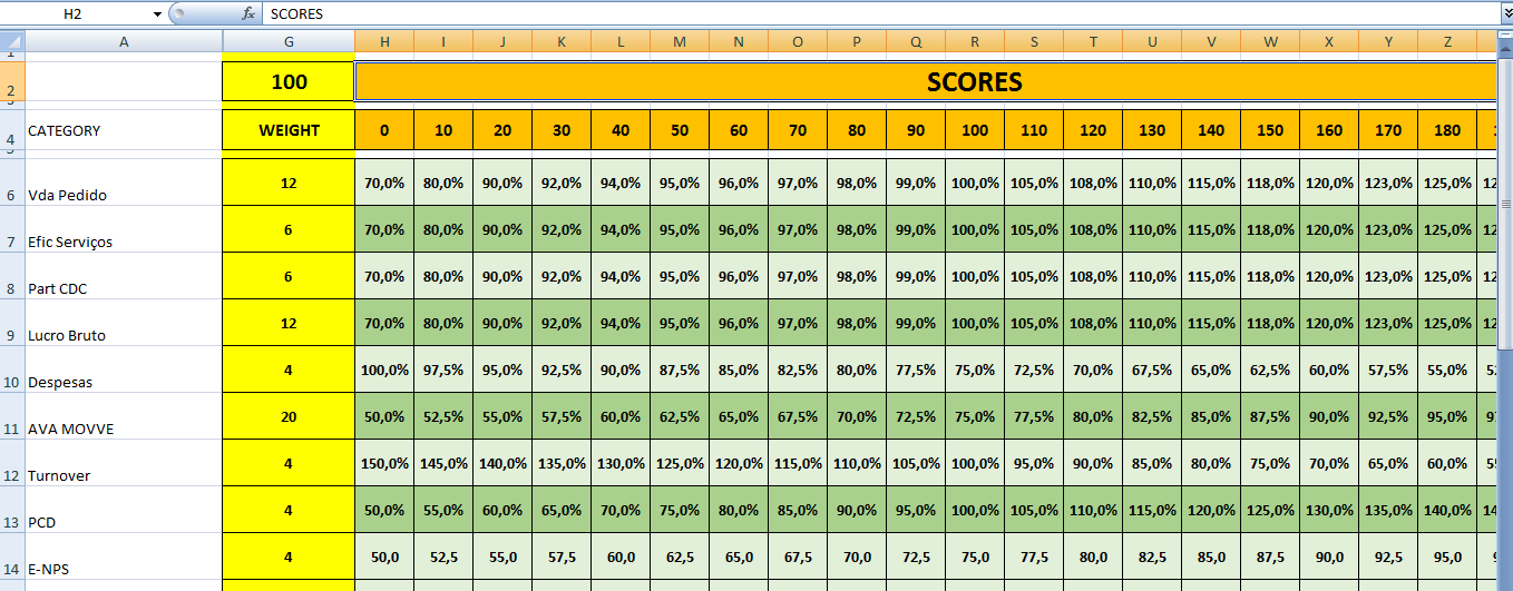
DATA SHEET

INFORMATION SHEET

So, what I want is a formula that finds the Category (let's do it for row 2 - category is "vda pedido") then it goes to the result (80,1%), which would be row 6 column I from the information sheet, so it should give me the score (which is in row 4 of information sheet), in this case that is 10 (row 4 column I)... Is it possible?

Note that the result needs to be between the right column of the score and the next column, it's not an exact match.

 

[Proezas]

.

 

[AhoyNC]

You can use INDEX & MATCH functions.
You will need to change the ranges in the formulas below to match your data.

To find the RESUT of Vda Pedido
=INDEX($I$2:$I$9,MATCH("Vda Pedido",$E$2:$E$9,0))

You will need to change both the ranges and the A1 in the formula below (change A1 to the cell that holds the above formula for result).
To get column header with score.

=INDEX($H$4:$Z$4,MATCH(A1,INDEX($H$6:$Z$12,MATCH("Vda Pedido",$A$6:$A$12,0),0)))

<colgroup><col style="width:48pt" width="64"> </colgroup><tbody>
</tbody>

The attached link should explain how to look up a column header.
https://www.youtube.com/watch?v=f2N0wkY9xLQ

 

[Proezas]

You can use INDEX & MATCH functions.
You will need to change the ranges in the formulas below to match your data.

To find the RESUT of Vda Pedido
=INDEX($I$2:$I$9,MATCH("Vda Pedido",$E$2:$E$9,0))

You will need to change both the ranges and the A1 in the formula below (change A1 to the cell that holds the above formula for result).
To get column header with score.

=INDEX($H$4:$Z$4,MATCH(A1,INDEX($H$6:$Z$12,MATCH("Vda Pedido",$A$6:$A$12,0),0)))

<tbody>
</tbody>

The attached link should explain how to look up a column header.
https://www.youtube.com/watch?v=f2N0wkY9xLQ

Thanks a lot! That's exactly what I was searching for and works almost fine.

I do have a little issue yet. Is there a way to know if the sorting of the line is smallest to biggest or biggest to smallest?

In my table I do have categories "Despesas" and "Turnover" which scores are sorted by biggest to smallest, so I got a little issue in the MATCH formula when because it's not a exact match, so I need to identify either if it's greater or lesser than the number. Is there a formula that identifies if the row is sorted one or other way so I can put everything in only one formula?

Right now I did it with and "=IF(OR(cell="Despesas";cell="Turnover"),INDEX(MATCH(INDEX(MATCH())),-1)), INDEX(MATCH(INDEX(MATCH())),1)))"

But if I have many other categories that are sorted this way I'll get some trouble needing to name them all.

 

[AhoyNC]

One way would be to add a helper column to your INFO sheet. The formula in the helper column will return a 1 for TRUE (sort in descending order) or a 0 for false (sort in ascending order). Then instead of hard coding in a category you could use a VLOOKUP as in cell B9 of the example below in your IF formula.

IF(VLOOKUP(B8,$A$3:$E$6,5,0),INDEX(MATCH(INDEX(MATCH())),-1)), INDEX(MATCH(INDEX(MATCH())),1)))

Excel Workbook
	A	B	C	D	E
1
2	Category	0	10	20	Helper
3	Vda	70%	80%	90%	0
4	Despesas	100%	97.50%	95%	1
5	Efic	70%	80%	90%	0
6	Turnover	150%	145%	135%	1
7
8	Find	Efic
9		0
Sheet

 

[Proezas]

One way would be to add a helper column to your INFO sheet. The formula in the helper column will return a 1 for TRUE (sort in descending order) or a 0 for false (sort in ascending order). Then instead of hard coding in a category you could use a VLOOKUP as in cell B9 of the example below in your IF formula.

IF(VLOOKUP(B8,$A$3:$E$6,5,0),INDEX(MATCH(INDEX(MATCH())),-1)), INDEX(MATCH(INDEX(MATCH())),1)))

*	A	B	C	D	E
1	*	*	*	*	*
2	Category	0	10	20	Helper
3	Vda	70%	80%	90%	0
4	Despesas	100%	97.50%	95%	1
5	Efic	70%	80%	90%	0
6	Turnover	150%	145%	135%	1
7	*	*	*	*	*
8	Find	Efic	*	*	*
9	*	0	*	*	*

<colgroup><col style="width:30px; "><col style="width:75px;"><col style="width:64px;"><col style="width:64px;"><col style="width:64px;"><col style="width:100px;"></colgroup><tbody>
</tbody>

Spreadsheet Formulas

Cell Formula E3 =IF(C3>B3,0,1) B9 =VLOOKUP(B8,$A$3:$E$6,5,0) <tbody> </tbody>

<tbody>
</tbody>

Excel tables to the web >> Excel Jeanie HTML 4

Certainly much better!

Thanks once again for your help! I believe this thread can be closed now.