Search array for all instances of a date, and criteria from separate column, return names from all matching rows

[DogWithWiFi]

Hey all, I can't figure out how to pull this off with a single formula, or what the best approach might be (FILTER, INDEX & MATCH, ?).

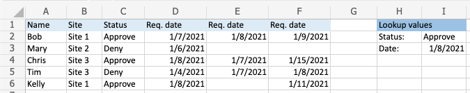
I want to return a list of Names (and the associated Status) from all rows where: Any of the dates in D:F match the dynamic date in I3 and the Status in C matches the dynamic value in I2.

In my example, the list should return:
Bob | Approve
Chris | Approve
Kelly | Approve

Any help is appreciated - thanks!

 

[StephenCrump]

Welcome to the Forum!

Try: =FILTER(A2:A6,(C2:C6=I2)*((D2:D6=I3)+(E2:E6=I3)+(F2:F6=I3)),"None found")

The status is redundant (it will always match I2), but if you must show it: =FILTER(A2:A6&" | "& I2,(C2:C6=I2)*((D2:D6=I3)+(E2:E6=I3)+(F2:F6=I3)),"None found")

 

[DogWithWiFi]

Hey Stephen, thanks for the welcome and the response!

I should have mentioned in my op that I have a version of your example working, but the dates in my live dataset are spread across ~50 columns (as opposed to just 3), so I thought I'd created a needlessly long formula, and was unaware of a "better" and/or more concise option. (If you think there is a better/more concise formula solution in this scenario, please let me know).

Thanks again - I very much appreciate your expert input (and am glad to know I wasn't way off the mark...)!

 

[StephenCrump]

=FILTER(A2:A6,(C2:C6=I2)*MMULT(--(D2:F6=I3),SEQUENCE(COLUMNS(D1:F1),,1,0)),"None found")

It's always better to give your full requirements up-front. For only three columns, I thought this would be overkill.

 

[DogWithWiFi]

Thanks again, Stephen (and apologies for any wasted time as a result of my oversight).

The most recent formula works perfectly on the sample data, but when I modified to correlate to my live data, something traced to the dates array (T:AN) is throwing up a persistent VALUE error. Haven't cracked it yet—all the date formatting looks to match—but I might be missing something obvious and will try again tomorrow...

=FILTER(Sheet1!$E$4:$E$5000,(Sheet1!$AO$4:$AO$5000=$I$2)*MMULT(--(Sheet1!$T$4:$AN$5000=$I$3),SEQUENCE(COLUMNS(Sheet1!T1:AN1),,1,0)),"None found")