Search in dynamic range

[kdew]

Hi all, I have the following problem to solve using Excel.

I have a list of sample numbers in one Excel file ('file 1' in attached file).

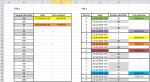
I have to couple each sample identifier from file 1 (cells in gray) to information from another sample of the same person ('file 2'). The information I need should be imported in columns C and D (which has been partially filled in for clarity).

The information from file 2 that I need concerns 1) the test outcome (column I), and 2) the test Date (column G), that belongs to the same person (column F) as the sample identifier belongs to. However, the information I need is NEVER on the same row as the gray sample identifiers, but must be extracted from columns G & I on the row where either 'Positive' or 'Negative' is in column H.

For instance, for sample 2 (and 11 and 3) I need 'Negative' from position I22 and the corresponding date in G22. For Sample 16, I need 'Negative' from I11 and date from G11.

I know how to retrieve cell content from a given relative position using INDEX and MATCH functions:
=INDEX('K:\[file1.xlsx]Tab1'!$A$1:$B$10000;MATCH(A1;'K:\file2.xlsx]Tab2'!$A$1:$A$10000;0);2)

However, the difficulty here is that I need to lookup for every sample identifier, the test outcome and date from the row where test outcome (column I) is NOT "-" for the SAME person, given in column F.

An extra difficulty would be that for person A there are multiple rows where there is not "-" in column I, and I'd need in different columns both of the test outcomes (I5 and I9) and both the dates (G5 and G9).

Any help about how to approach this is much appreciated.

I have also posted this thread on Excelforum: How to search within a dynamic range

 

[KRice]

Welcome to the forum.

Have a look at this and see if it will work. Inputs are in B27 and down, and the corresponding person, the number of entries to find, and the date/outcome combinations spill over into the columns to the right. If this is close, then the range references will need to be modified to point to the correct files, worksheets, and ranges in your setup. This is configured to find up to three entries in any given "person" block. If more than three entries (i.e., positives + negatives) are present, then simply copy the last two columns (the Date and Test Outcome results table) and paste them immediately to the right to create new receiver cells for a 4th entry, and so on. This approach finds the data matching the criteria you've described, but it does not carry over the cell fill color...I believe VBA would be needed to do that efficiently.

Example Excel file.xlsx
	A	B	C	D	E	F	G	H	I	J
1
2		File 1				File 2
3
4		Sample identifier	Date	Test outcome		Person	Date	Sample identifier	Test outcome
5		16	10/17/2019 3:30	NEGATIVE		A	12/13/2019 7:45	18	POSITIVE
6		200				A	10/14/2019 4:00	10	-
7		21	10/18/2019 4:30	POSITIVE		A	11/14/2019 7:10	7	-
8		0				A	10/15/2019 3:55	19	-
9		13	…	…		A	11/15/2019 7:20	9	NEGATIVE
10		15	…	…		B	10/16/2019 4:05	8	-
11		300				B	10/17/2019 3:30	4	NEGATIVE
12		400				B	12/17/2019 7:50	16	-
13		2	…	…		C	10/18/2019 4:30	1	POSITIVE
14		500				C	10/19/2019 4:30	21	-
15		11				D	11/18/2019 8:20	5	POSITIVE
16		600				E	10/19/2019 3:35	13	-
17		3				E	10/20/2019 3:35	15	-
18		6				F	11/20/2019 7:25	12	-
19		700				F	12/20/2019 7:50	2	-
20		16				F	10/21/2019 3:25	11	-
21		800				F	10/22/2019 3:00	3	-
22		19				F	11/22/2019 9:40	17	NEGATIVE
23		10				G	10/23/2019 4:15	14	POSITIVE
24		1000				H	12/23/2019 7:45	6	-
25
26		Sample ID	Person	Count	Date	Test Outcome	Date	Test Outcome	Date	Test Outcome
27		1	C	1	10/18/19 4:30	POSITIVE
28		2	F	1	11/22/19 9:40	NEGATIVE
29		3	F	1	11/22/19 9:40	NEGATIVE
30		4	B	1	10/17/19 3:30	NEGATIVE
31		5	D	1	11/18/19 8:20	POSITIVE
32		6	H	0	no match	no match
33		7	A	2	12/13/19 7:45	POSITIVE	11/15/19 7:20	NEGATIVE
34		8	B	1	10/17/19 3:30	NEGATIVE
35		9	A	2	12/13/19 7:45	POSITIVE	11/15/19 7:20	NEGATIVE
36		10	A	2	12/13/19 7:45	POSITIVE	11/15/19 7:20	NEGATIVE
37		11	F	1	11/22/19 9:40	NEGATIVE
38		12	F	1	11/22/19 9:40	NEGATIVE
Blad1

Cell Formulas
Range	Formula
C27:C38	C27	=IFERROR(INDEX($F$5:$F$24,MATCH($B27,$H$5:$H$24,0)),"no match")
D27:D38	D27	=COUNTIFS($F$5:$F$24,C27,$I$5:$I$24,"<>-")
E27:E38	E27	=IF($D27=0,"no match",INDEX($G$5:$G$24,AGGREGATE(15,6,(ROW($G$5:$G$24)-ROW($G$4))/(($F$5:$F$24=$C27)*($I$5:$I$24<>"-")),INT((COLUMNS($E$26:E$26)-1)/2)+1)))
F27:F38	F27	=IF($D27=0,"no match",INDEX($I$5:$I$24,AGGREGATE(15,6,(ROW($G$5:$G$24)-ROW($G$4))/(($F$5:$F$24=$C27)*($I$5:$I$24<>"-")),INT((COLUMNS($E$26:F$26)-1)/2)+1)))
G27:G38,I27:I38	G27	=IFERROR(INDEX($G$5:$G$24,AGGREGATE(15,6,(ROW($G$5:$G$24)-ROW($G$4))/(($F$5:$F$24=$C27)*($I$5:$I$24<>"-")),INT((COLUMNS($E$26:G$26)-1)/2)+1)),"")
H27:H38,J27:J38	H27	=IFERROR(INDEX($I$5:$I$24,AGGREGATE(15,6,(ROW($G$5:$G$24)-ROW($G$4))/(($F$5:$F$24=$C27)*($I$5:$I$24<>"-")),INT((COLUMNS($E$26:H$26)-1)/2)+1)),"")

 

[kdew]

Hi KRice. Many thanks for your reply. Yes, this effectively solves the problem.
Thanks a lot!

 

[KRice]

Great news! You're welcome...and I appreciate the feedback.