Separate sections custom sort - numbers with text separate sections

[butch3]

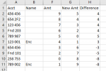
I've attached two images that will help visualize what I'm trying to do. I have 4 different types of data that need to be sorted. In the 'example' image, you can see that the accounts (Col A) is all clumped together. The 'output' image shows what I would like to happen. The number of data elements will change for each spreadsheet (macro) I would run the code on. Highlighting of the two sums preferred.

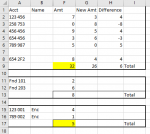
The first section in 'output' is for the accounts that are only numbers. The second sections is for accounts that have letters after the first 3 digits.

A Sum is produced for a combined total of the values in the Amt Column.

Next, when the first three digits are 'Fnd'. Total is produced for this section. The numbers to the right of the Amt column is removed.

Lastly, if the Name Column is named 'Enc' the row would be placed in this section. An alternate way to code this is to evaluate whether the 5th and 6th digit is 0 if it is, the row transfers into the last section and a sum for this section is produced. The numbers to the right of the Amt column is removed.

Note, each section is sorted by the Account without any sorting into any other section.


Example:

Book1
	A	B				F	G	H
1	Acct	Name				Amt	New Amt	Difference
2	456 456					9	5	4
3	654 2F2					8	4	4
4	123 456					7	3	4
5	Fnd 203					6	2	4
6	789 987					5	0	5
7	123 001	Enc				4	1	3
8	654 456					3	6	-3
9	Fnd 101					2	7	-5
10	258 753					0	8	-8
11	789 002	Enc				1	9	-8
Sheet1

After Macro Output:

Book1
	A	B				F	G	H	I
1	Acct	Name				Amt	New Amt	Difference
2	123 456					7	3	4
3	258 753					0	8	-8
4	456 456					9	5	4
5	654 456					3	6	-3
6	789 987					5	0	5
7
8	654 2F2					8	4	4
9						32	26	6	Total
10
11	Fnd 101					2
12	Fnd 203					6
13						8			Total
14
15	123 001	Enc				4
16	789 002	Enc				1
17						5			Total
Sheet1

 

[DanteAmor]

Check all decimals.
You could paste the original data here to review.

 

[butch3]

Okay. So I ran the code in a totally new sheet with no other code other than yours (I only changed the Enc and Vou so that it was capitalized fully and I'm showing that it is labeling not balanced when it should be balanced. And the weird thing is I have changed "Not Balanced" to wtot and also to .Value, and it is picking up the correct values to compare to....

Example:

Book1
	A	B	C	D	E	F	G	H
1	Account	Description				ENC	RBR	Difference
2	101 12ST037924	17/18 PAVEMENT				11,560.43	11560.43	0
3	101 2100001	ENCUMBRANCES				-11,560.43		-4,631,281.61
4	101 2100002	VOUCHERS PAYABL				-124,946.14		-512,106.45
5	203 12ST038924	2019 PAVE				9,191.04	9191.04	0
6	203 2100001	ENCUMBRANCES				-246,522.54		-949,060.22
7	203 4636267	HORTICULTURAL -				228,265.75	228265.75	0
8	203 4785763	REPL-EQUIPMENT				9,065.75	9065.75	0
9	206 2100001	ENCUMBRANCES				-830,704.98
10	206 12ST036924	16/17 PAVEMENT				9,091.50	9091.5	0
11	206 12ST037924	17/18 PAVEMENT				821,613.48	821613.48	0
12	361 2100001	ENCUMBRANCES				-221,226.50
13	361 4541901D	MAPS (TPM/TTPM)				129,750.00		129,750.00
14	361 4541901S	MAPS (TPM/TTPM)				91,476.50	91476.5	0
15	999 9999999	SUSPENSE ACCOUN				124,946.14	-23245.75	148,191.89
16	Fnd 101 GEN	Fund				-8,294.03		-8,294.03
17	Fnd 207 PRO	Fund				-4,731.00		-4,731.00
18	Fnd 212 MEA	Fund				13,025.03		13,025.03
Sheet1

Output:

Book1
	A	B	C	D	E	F	G	H
1
2	203 4636267	HORTICULTURAL -				228265.75	228265.75	0
3	203 4785763	REPL-EQUIPMENT				9065.75	9065.75	0
4	361 4541901D	MAPS (TPM/TTPM)				129750		129750
5	361 4541901S	MAPS (TPM/TTPM)				91476.5	91476.5	0
6	999 9999999	SUSPENSE ACCOUN				124946.14	-23245.75	148191.89
7
8	101 12ST037924	17/18 PAVEMENT				11560.43	11560.43	0
9	203 12ST038924	2019 PAVE				9191.04	9191.04	0
10	206 12ST036924	16/17 PAVEMENT				9091.5	9091.5	0
11	206 12ST037924	17/18 PAVEMENT				821613.48	821613.48	0
12		Total				1434960.59	1157018.7	277941.89
13								Not Balanced
14
15	Fnd 101 GEN	Fund				-8294.03
16	Fnd 207 PRO	Fund				-4731
17	Fnd 212 MEA	Fund				13025.03
18		Total				0
19						Balanced
20
21	101 2100001	ENCUMBRANCES				-11560.43
22	101 2100002	VOUCHERS PAYABL				-124946.14
23	203 2100001	ENCUMBRANCES				-246522.54
24	206 2100001	ENCUMBRANCES				-830704.98
25	361 2100001	ENCUMBRANCES				-221226.5
26		Total				-1434960.59
27						Not Balanced
Sheet2

 

[butch3]

I wondering if you're test reproduces the same issue?

So I ran the code as

If wtot + .Value = 0 Then .Offset(1).Value = "Balanced" Else .Offset(1).Value = .Value + wtot

and the output for that cell was

so it seems it might be a rounding error?

 

[butch3]

I'm not sure if its the best idea fundamentally to round the absolute value of wtot + .Value but wouldn't that solve the issue?

I wondering if you're test reproduces the same issue?

So I ran the code as

If wtot + .Value = 0 Then .Offset(1).Value = "Balanced" Else .Offset(1).Value = .Value + wtot

and the output for that cell was View attachment 5942 so it seems it might be a rounding error?

 

[DanteAmor]

I add this and works:

If Val(wtot) + Val(.Value) = 0

Try this:

Option Explicit

Dim b As Variant, c As Variant, d As Variant, e As Variant, wtot As Double

Sub Separate_sections()
  Dim a As Variant, sh1 As Worksheet, sh2 As Worksheet
  Dim i As Long, nb As Long, nc As Long, nd As Long, ne As Long
  Dim lr As Long, lr2 As Long, m
  
  Application.ScreenUpdating = False
  
  Set sh1 = Sheets("Sheet1")
  Set sh2 = Sheets("Sheet2")
  sh2.Rows("2:" & Rows.Count).ClearContents
  a = sh1.Range("A2:H" & sh1.Range("A" & Rows.Count).End(xlUp).Row).Value2
  
  ReDim b(1 To UBound(a), 1 To 8)
  ReDim c(1 To UBound(a), 1 To 8)
  ReDim d(1 To UBound(a), 1 To 6)
  ReDim e(1 To UBound(a), 1 To 6)
  
  For i = 1 To UBound(a)
    m = Split(a(i, 1), " ")(1)
    m = Left(m, Len(m) - 1)
    Select Case True
      Case UCase(Left(a(i, 2), 3)) = UCase("Enc"), UCase(Left(a(i, 2), 3)) = UCase("Vou")
        ne = ne + 1
        Call fillarray(a, i, e, ne, 6)
      Case UCase(Left(a(i, 1), 3)) = UCase("Fnd")
        nd = nd + 1
        Call fillarray(a, i, d, nd, 6)
      Case IsNumeric(m)
        nb = nb + 1
        Call fillarray(a, i, b, nb, 8) '
      Case Else
        nc = nc + 1
        Call fillarray(a, i, c, nc, 8)
    End Select
  Next
  
  If nb > 0 Then Call FillSheet(sh2, 2, 2, b, nb, 8, False, "H", 0)
  
  lr = sh2.Range("A" & Rows.Count).End(xlUp).Row + 2
  If nc > 0 Then Call FillSheet(sh2, 2, lr, c, nc, 8, True, "H", 1)
  
  lr = sh2.Range("A" & Rows.Count).End(xlUp).Row + 4
  If nd > 0 Then Call FillSheet(sh2, lr, lr, d, nd, 6, True, "F", 0)
  
  lr = sh2.Range("A" & Rows.Count).End(xlUp).Row + 4
  If ne > 0 Then Call FillSheet(sh2, lr, lr, e, ne, 6, True, "F", 2)
End Sub

Sub FillSheet(sh2 As Worksheet, ini As Long, nRow As Long, ary As Variant, _
              nx As Long, col As Long, bFormula As Boolean, cf As String, x As Long)
  Dim lr2 As Long
  sh2.Range("A" & nRow).Resize(nx, col).Value = ary
  sh2.Range("A" & nRow).Resize(nx, col).sort key1:=sh2.Range("A" & nRow), order1:=xlAscending, Header:=xlNo
  If bFormula Then
    lr2 = sh2.Range("A" & Rows.Count).End(xlUp).Row + 1
    With sh2.Range("F" & lr2 & ":" & cf & lr2)
      .Formula = "=SUM(F" & ini & ":F" & lr2 - 1 & ")"
      .Value = .Value
      If x = 1 Then
        wtot = sh2.Range("F" & lr2).Value
      End If
    End With
    sh2.Range("B" & lr2).Value = "Total"
    With sh2.Range(cf & lr2)
      Select Case x
        Case 0, 1
          If .Value = 0 Then .Offset(1).Value = "Balanced" Else .Offset(1).Value = "Not Balanced"
        Case Else
          If Val(wtot) + Val(.Value) = 0 Then .Offset(1).Value = "Balanced" Else .Offset(1).Value = "Not Balanced"
      End Select
    End With
  End If
End Sub

Sub fillarray(a As Variant, i As Long, Arr As Variant, n As Long, m As Long)
  Dim j As Long
  For j = 1 To m
    Arr(n, j) = a(i, j)
  Next
End Sub

 

[butch3]

Works. The other issue I had, I just resolved it.

I add this and works:

If Val(wtot) + Val(.Value) = 0

 

[DanteAmor]

I guess then everything is covered. Let me know any questions.
I'm glad to help you.