Set a criterion then check against that criteria

Samgraphics

Board Regular
Joined
Jan 9, 2022
Messages
52
Office Version
  1. 2011
Platform
  1. MacOS
Hi,.
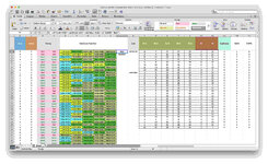
I am trying to rate a combination of numbers based on the criteria I create but there are more than one criterion. Say for example a combination of numbers has 1 low odd, 2 high odds, and 2 high evens I would like to put a ratting in the column next to it like "good" if I think that's a good combination or "bad" if I think it's a bad combination. But what I'm checking will not be the actual numbers, but the text that represents numbers. I'm wondering if there is a way to check/filter the results to see how many lowodds/highodds/higheven/lowevens there are in each 5 number combination and return either good/bad based on the criteria I set. Something like =IF(C2:E2="LOW ODD"*2&"HIGH ODD"*1&"HIGH EVEN"*2,"GOOD","BAD") I know I can't use SUMPRODUCT because the value in each cell is not a number but I'm lost as to how to solve this.

Thank you again for all your help
 

Attachments

  • Screen Shot 2022-01-20 at 3.16.15 AM.jpg
    Screen Shot 2022-01-20 at 3.16.15 AM.jpg
    142.1 KB · Views: 15

Excel Facts

Enter current date or time
Ctrl+: enters current time. Ctrl+; enters current date. Use Ctrl+: Ctrl+; Enter for current date & time.
Hi,

I'm unclear what your question is, do you mean LOW ODD, HIGH ODD, etc. represent numbers or you want to Count how many of them are in the 5 cells?

May be this?

Book3.xlsx
OPQRST
2LOW ODDHIGH EVENHIGH ODDHIGH ODDHIGH ODDBad
Sheet941
Cell Formulas
RangeFormula
T2T2=IF(AND(COUNTIF(O2:S2,"Low odd")=2,COUNTIF(O2:S2,"High odd")=1,COUNTIF(O2:S2,"High even")=2),"Good","Bad")
 
Upvote 0
Hi,

I'm unclear what your question is, do you mean LOW ODD, HIGH ODD, etc. represent numbers or you want to Count how many of them are in the 5 cells?

May be this?

Book3.xlsx
OPQRST
2LOW ODDHIGH EVENHIGH ODDHIGH ODDHIGH ODDBad
Sheet941
Cell Formulas
RangeFormula
T2T2=IF(AND(COUNTIF(O2:S2,"Low odd")=2,COUNTIF(O2:S2,"High odd")=1,COUNTIF(O2:S2,"High even")=2),"Good","Bad")
Hi jtakw,
Thank you for your reply and solution. Yes, this is what I was looking for or something like that anyway, but I think I confused myself that's why my question was so confusing to you too.

This solution is working perfectly, but I realize that it isn't achieving my ultimate goal, NO FAULT OF YOURS, it's just that I wasn't clear in my question. That's totally on me!

That is part of what I need, however, I would like to have at least 3 - 4 different criteria that it will check each combination against. for example,
1. 1-low odd, 2-high odd, 2-high even - "good"
2. 1-low even 2-high even 2-high odd - "good"
3. 2-low odd, 1-high odd 2-high even - "average"
4. 2-low even 1-high even 2-high odd - "average"
excel would check each combination against these 4 criteria and then if it has a combination that meets any of these criteria have it say "good","average", and if it doesn't then "bad" actually.

Please help me figure out how to go about doing that.

Thank you
 
Upvote 0
This should work, test it against your data and see if the results are correct:

Book3.xlsx
OPQRST
2LOW ODDHIGH EVENHIGH ODDHIGH ODDHIGH ODDBad
3LOW ODDHIGH ODDHIGH ODDHIGH EVENHIGH EVENGood
4LOW EVENHIGH EVENHIGH EVENHIGH ODDHIGH ODDGood
5LOW ODDLOW ODDHIGH ODDHIGH EVENHIGH EVENAverage
6LOW EVENLOW EVENHIGH EVENHIGH ODDHIGH ODDAverage
Sheet941
Cell Formulas
RangeFormula
T2:T6T2=IF(AND(OR(COUNTIF(O2:S2,{"Low odd","Low even"})=1),AND(COUNTIF(O2:S2,{"High odd","High even"})=2)),"Good",IF(OR(AND(COUNTIF(O2:S2,"Low odd")=2,COUNTIF(O2:S2,"High odd")=1,COUNTIF(O2:S2,"High even")=2),AND(COUNTIF(O2:S2,"Low even")=2,COUNTIF(O2:S2,"High even")=1,COUNTIF(O2:S2,"High odd")=2)),"Average","Bad"))
 
Upvote 0
Solution
This should work, test it against your data and see if the results are correct:

Book3.xlsx
OPQRST
2LOW ODDHIGH EVENHIGH ODDHIGH ODDHIGH ODDBad
3LOW ODDHIGH ODDHIGH ODDHIGH EVENHIGH EVENGood
4LOW EVENHIGH EVENHIGH EVENHIGH ODDHIGH ODDGood
5LOW ODDLOW ODDHIGH ODDHIGH EVENHIGH EVENAverage
6LOW EVENLOW EVENHIGH EVENHIGH ODDHIGH ODDAverage
Sheet941
Cell Formulas
RangeFormula
T2:T6T2=IF(AND(OR(COUNTIF(O2:S2,{"Low odd","Low even"})=1),AND(COUNTIF(O2:S2,{"High odd","High even"})=2)),"Good",IF(OR(AND(COUNTIF(O2:S2,"Low odd")=2,COUNTIF(O2:S2,"High odd")=1,COUNTIF(O2:S2,"High even")=2),AND(COUNTIF(O2:S2,"Low even")=2,COUNTIF(O2:S2,"High even")=1,COUNTIF(O2:S2,"High odd")=2)),"Average","Bad"))

jtakw THANK YOU SO MUCH! REALLY!​


I DON'T REALLY UNDERSTAND THE ENTIRE FORMULA BUT IT IS WORKING PERFECTLY. IF I DID WANT TO CHANGE THE CRITERION, I DON'T THINK I UNDERSTAND IT ENOUGH TO ADJUST IT BUT I APPRECIATE YOUR HELP SO MUCH. THANK YOU.

FROM WHAT I CAN SEE THE FORMULA ISN'T WRITTEN LITERALLY AS THE CRITERION I GAVE YOU, PLEASE TELL ME IF I'M READING IT CORRECTLY.
IF O2 TO S2 HAS A LOW ODD OR LOW EVEN AND IF O2 TO S2 HAS TWO HIGH ODD OR TWO HIGH EVEN THEN IT'S GOOD.
IF O2 TO S2 HAS TWO LOW ODD, ONE HIGH ODD OR ONE HIGH EVEN, AND TWO LOW EVEN THEN IT'S AVERAGE.
IF IT DOESN'T HAVE ANY OF THE ABOVE IT'S BAD.
IS THAT CORRECT?
I REALLY WISH I COULD UNDERSTAND IT BETTER IN CASE I NEED TO SET A NEW CRITERION OR CHANGE AN EXISTING ONE.

THANK YOU VERY MUCH.
 
Upvote 0
You're welcome, thanks for the feedback, glad it works for you.

Actually, my formula IS written Exactly according to your requirements as described:

1. 1-low odd, 2-high odd, 2-high even - "good"
2. 1-low even 2-high even 2-high odd - "good"
3. 2-low odd, 1-high odd 2-high even - "average"
4. 2-low even 1-high even 2-high odd - "average"
excel would check each combination against these 4 criteria and then if it has a combination that meets any of these criteria have it say "good","average", and if it doesn't then "bad" actually.

It is important to follow the Order of the Nested ANDs and ORs to understand the formula properly.
 
Upvote 0
You're welcome, thanks for the feedback, glad it works for you.
Actually, my formula IS written Exactly according to your requirements as described:


It is important to follow the Order of the Nested ANDs and ORs to understand the formula properly.
HI, YES YOU'RE RIGHT ACTUALLY, THAT'S MY MISTAKE AS I UNDERSTOOD THE FORMULA WRONG.:)SORRY. THANKS AGAIN SO MUCH FOR ALL THE HELP AND TIME TO RESPOND TO MY MESSAGES. YOU'VE BEEN A HUGE HELP. THANK YOU.
 
Upvote 0

Forum statistics

Threads
1,214,651
Messages
6,120,744
Members
448,989
Latest member
mariah3

We've detected that you are using an adblocker.

We have a great community of people providing Excel help here, but the hosting costs are enormous. You can help keep this site running by allowing ads on MrExcel.com.
Allow Ads at MrExcel

Which adblocker are you using?

Disable AdBlock

Follow these easy steps to disable AdBlock

1)Click on the icon in the browser’s toolbar.
2)Click on the icon in the browser’s toolbar.
2)Click on the "Pause on this site" option.
Go back

Disable AdBlock Plus

Follow these easy steps to disable AdBlock Plus

1)Click on the icon in the browser’s toolbar.
2)Click on the toggle to disable it for "mrexcel.com".
Go back

Disable uBlock Origin

Follow these easy steps to disable uBlock Origin

1)Click on the icon in the browser’s toolbar.
2)Click on the "Power" button.
3)Click on the "Refresh" button.
Go back

Disable uBlock

Follow these easy steps to disable uBlock

1)Click on the icon in the browser’s toolbar.
2)Click on the "Power" button.
3)Click on the "Refresh" button.
Go back
Back
Top